- Intuition For Tree Indexes
- Indexed Sequential Access Method (ISAM)
- B+ Trees: A Dynamic Index Structure
- Search
- Insert
- Delete
- Duplicates
- B+ Trees in Practice
We now consider two index data structures, called ISAM and B+ trees, based on tree organizations. These structures provide efficient support for range searches, including sorted file scans as a special case. Unlike sorted files, these index structures support efficient insertion and deletion. They also provide support for equality selections, although they are not as efficient in this case as hash-based indexes. An ISAM(Indexed Sequential Access Method) tree is a static index structure that is effective when the file is not frequently updated, but it is unsuitable for files that grow and shrink a lot. The B+ tree is a dynamic structure that adjusts to changes in the file gracefully. It is the most widely used index structure because it adjusts well to changes and supports both equality and range queries. Notation: In the ISAM and B+ tree structures, leaf pages contain data entries. For convenience, we denote a data entry with search key value k as k*. Non-leaf pages contain index entries of the form (search key Value, page id) and are used to direct the search for a desired data entry (which is stored in some leaf). We often simply use entry where the context makes the nature of the entry (index or data) clear.
Intuition For Tree Indexes
Consider a file of Students records sorted by gpa. To answer a range selection such as “Find all students with a gpa higher than 3.0,” we must identify the first such student by doing a binary search of the file and then scan the file from that point on. If the file is large, the initial binary search can be quite expensive, since cost is proportional to the number of pages fetched; can we improve upon this method?
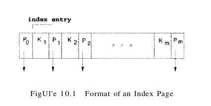
One idea is to create a second file with one record per page in the original (data) file, of the form (first key on page, pointer to page), again sorted by the key attribute (which is gpa in our example). The format of a page in the second index file is illustrated in Figure 10.1. We refer to pairs of the form (key, pointer) as index entries or just entries when the context is clear. Note that each index page contains one pointer more than the number of keys – each key serves as a separator – for the contents of the pages pointed to by the pointers to its left and right.
The simple index file data structure is illustrated in Figure 10.2.

We can do a binary search of the index file to identify the page containing the first key (gpa) value that satisfies the range selection (in our example, the first student with gpa over 3.0) and follow the pointer to the page containing the first data record with that key value. We can then scan the data file sequentially from that point on to retrieve other qualifying records. This example uses the index to find the first data page containing a Students record with gpa greater than 3.0, and the data file is scanned from that point on to retrieve other such Students records. Because the size of an entry in the index file (key value and page id) is likely to be much smaller than the size of a page, and only one such entry exists per page of the data file, the index file is likely to be much smaller than the data file; therefore, a binary search of the index file is much faster than a binary search of the data file. However, a binary search of the index file could still be fairly expensive, and the index file is typically still large enough to make inserts and deletes expensive. The potential large size of the index file motivates the tree indexing idea: Why not apply the previous step of building an auxiliary structure all the collection of index records and so on recursively until the smallest auxiliary structure fits on one page? This repeated construction of a one-level index leads to a tree structure with several levels of non-leaf pages.
Indexed Sequential Access Method (ISAM)
The ISAM data structure is illustrated in Figure 10.3. The data entries of the ISAM index are in the leaf pages of the tree and additional overflow pages chained to some leaf page. Database systems carefully organize the layout of pages so that page boundaries correspond closely to the physical characteristics of the underlying storage device. The ISAM structure is completely static (except for the overflow pages, of which it is hoped, there will be few) and facilitates such low-level optimizations.
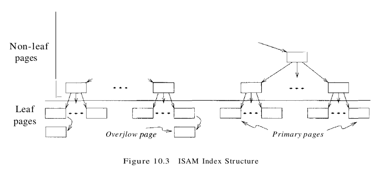
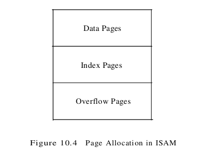
Each tree node is a disk page, and all the data resides in the leaf pages. This corresponds to an index that uses Alternative (1) for data entries. we can create an index with Alternative (2) by storing the data records in a separate file and storing (key, rid) pairs in the leaf pages of the ISAM index. When the file is created, all leaf pages are allocated sequentially and sorted on the search key value. (If Alternative (2) or (3) is used, the data records are created and sorted before allocating the leaf pages of the ISAM index.) The non-leaf level pages are then allocated. If there are several inserts to the file subsequently, so that more entries are inserted into a leaf than will fit onto a single page, additional pages are needed because the index structure is static. These additional pages are allocated from an overflow area. The allocation of pages is illustrated in Figure 10.4.
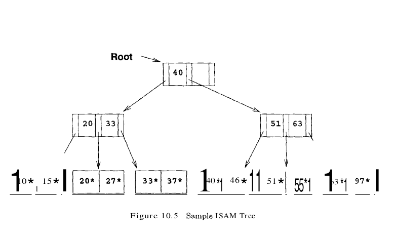
The basic operations of insertion, deletion, and search are all quite straightforward. For an equality selection search, we start at the root node and determine which subtree to search by comparing the value in the search field of the given record with the key values in the node. (The search algorithm is identical to that for a B+ tree.) For a range query, the starting point in the data (or leaf) level is determined similarly, and data pages are then retrieved sequentially. For inserts and deletes, the appropriate page is determined as for a search, and the record is inserted or deleted with overflow pages added if necessary. The following example illustrates the ISAM index structure. Consider the tree shown in Figure 10.5. All searches begin at the root. For example, to locate a record with the key value 27, we start at the root and follow the left pointer, since 27 < 40. We then follow the middle pointer, since 20 < 27 < 33. For a range search, we find the first qualifying data entry as for an equality selection and then retrieve primary leaf pages sequentially (also retrieving overflow pages as needed by following pointers from the primary pages). The primary leaf pages are assumed to be allocated sequentially. This assumption is reasonable because the number of such pages is known when the tree is created and does not change subsequently under inserts and deletes-and so no next leaf page pointers are needed. We assume that each leaf page can contain two entries. If we now insert a record with key value 23, the entry 23* belongs in the second data page, which already contains 20* and 27* and has no more space. We deal with this situation by adding an overflow page and putting 23* in the overflow page. Chains of overflow pages can easily develop. For instance, inserting 48*, 41*, and 42* leads to an overflow chain of two pages. The tree of Figure 10.5 with all these insertions is shown in Figure 10.6. The deletion of an entry k* is handled by simply removing the entry. If this entry is on an overflow page and the overflow page becomes empty, the page can be removed. If the entry is on a primary page and deletion makes the primary page empty, the simplest approach is to simply leave the empty primary page as it is; it serves as a placeholder for future insertions (and possibly non-empty overflow pages, because we do not move records from the overflow pages to the primary page when deletions on the primary page create space). Thus, the number of primary leaf pages is fixed at file creation time.

Note that, once the ISAM file is created, inserts and deletes affect only the contents of leaf pages. A consequence of this design is that long overflow chains could develop if a number of inserts are made to the same leaf. These chains can significantly affect the time to retrieve a record because the overflow chain has to be searched as well when the search gets to this leaf. (Although data in the overflow chain can be kept sorted, it usually is not, to make inserts fast.) To alleviate this problem, the tree is initially created so that about 20 percent of each page is free. However, once the free space is filled in with inserted records, unless space is freed again through deletes, overflow chains can be eliminated only by a complete reorganization of the file. The fact that only leaf pages are modified also has an important advantage with respect to concurrent access. When a page is accessed, it is typically ‘locked’ by the requestor to ensure that it is not concurrently modified by other users of the page. To modify a page, it must be locked in ‘exclusive’ mode, which is permitted only when no one else holds a lock on the page. Locking can lead to queues of users (transactions, to be more precise) waiting to get access to a page. Queues can be a significant performance bottleneck, especially for heavily accessed pages near the root of an index structure. In the ISAM structure, since we know that index-level pages are never modified, we can safely omit the locking step. Not locking index-level pages is an important advantage of ISAM over a dynamic structure like a B+ tree. If the data distribution and size are relatively static, which means overflow chains are rare, ISAM might be preferable to B+ trees due to this advantage.
B+ Trees: A Dynamic Index Structure
A static structure such as the ISAM index suffers from the problem that long overflow chains can develop as the file grows, leading to poor performance. This problem motivated the development of more flexible, dynamic structures that adjust gracefully to inserts and deletes. The B+ tree search structure, which is widely used, is a balanced tree in which the internal nodes direct the search and the leaf nodes contain the data entries. Since the tree structure grows and shrinks dynamically, it is not feasible to allocate the leaf pages sequentially as in ISAM, where the set of primary leaf pages was static. To retrieve all leaf pages efficiently, we have to link them using page pointers. By organizing them into a doubly linked list, we can easily traverse the sequence of leaf pages (sometimes called the sequence set) in either direction. This structure is illustrated in Figure 10.7.

The following are some of the main characteristics of a B+ tree:
- Operations (insert, delete) on the tree keep it balanced.
- A minimum occupancy of 50 percent is guaranteed for each node except the root if the deletion algorithm discussed later is implemented. However, deletion is often implemented by simply locating the data entry and removing it, without adjusting the tree as needed to guarantee the 50 percent occupancy, because files typically grow rather than shrink.
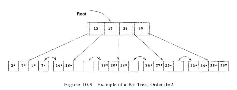
- Searching for a record requires just a traversal from the root to the appropriate leaf. We refer to the length of a path from the root to a leaf–any leaf, because the tree is balanced as the height of the tree. For example, a tree with only a leaf level and a single index level, such as the tree shown in Figure 10.9, has height 1, and a tree that has only the root node has height O. Because of high fan-out, the height of a B+ tree is rarely more than 3 or 4.
We will study B+ trees in which every node contains m entries, where $d \leq m \leq 2d$. The value d is a parameter of the B+ tree, called the order of the tree, and is a measure of the capacity of a tree node. The root node is the only exception to this requirement on the number of entries; for the root, it is simply required that $1 \leq m \leq 2d$
If a file of records is updated frequently and sorted access is important, maintaining a B+ tree index with data records stored as data entries is almost always superior to maintaining a sorted file. For the space overhead of storing the index entries, we obtain all the advantages of a sorted file plus efficient insertion and deletion algorithms. B+ trees typically maintain 67 percent space occupancy. B+ trees are usually also preferable to ISAM indexing because inserts are handled gracefully without overflow chains. However, if the dataset size and distribution remain fairly static, overflow chains may not be a major problem. In this case, two factors favor ISAM: the leaf pages are allocated in sequence (making scans over a large range more efficient than in a B+ tree, in which pages are likely to get out of sequence on disk over time, even if they were in sequence after bulk-loading), and the locking overhead of ISAM is lower than that for B+ trees. As a general rule, however, B+ trees are likely to perform better than ISAM.
Search
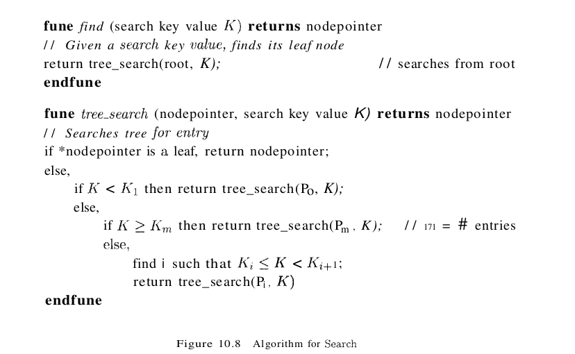
The algorithm for search finds the leaf node in which a given data entry belongs. A pseudocode sketch of the algorithm is given in Figure 10.8. We use the notation *ptr to denote the value pointed to by a pointer variable ptr and & (value) to denote the address of value. Note that finding i in tree_search requires us to search within the node, which can be done with either a linear search or a binary search (e.g., depending on the number of entries in the node). In discussing the search, insertion, and deletion algorithms for B+ trees, we assume that there are no duplicates. That is, no two data entries are allowed to have the same key value. Of course, duplicates arise whenever the search key does not contain a candidate key and must be dealt with in practice.
Consider the sample B+ tree shown in Figure 10.9. This B+ tree is of order d=2. That is, each node contains between 2 and 4 entries. Each non-leaf entry is a (key value, nodepointer) pair; at the leaf level, the entries are data records that we denote by k*. To search for entry 5*, we follow the left-most child pointer, since 5 < 13. To search for the entries 14* or 15*, we follow the second pointer, since 13 < 14 < 17, and 13 < 15 < 17. (We do not find 15* on the appropriate leaf and can conclude that it is not present in the tree.) To find 24*, we follow the fourth child pointer, since $24 \leq 24 < 30$.
Insert
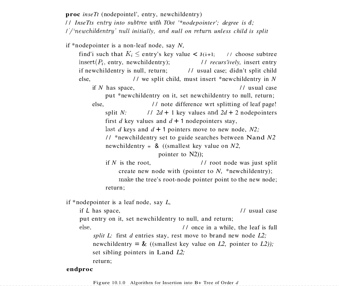
The algorithm for insertion takes an entry, finds the leaf node where it belongs, and inserts it there. Pseudocode for the B+ tree insertion algorithm is given in Figure 10.10. The basic idea behind the algorithm is that we recursively insert the entry by calling the insert algorithm on the appropriate child node. Usually, this procedure results in going down to the leaf node where the entry belongs, placing the entry there, and returning all the way back to the root node. Occasionally a node is full and it must be split. When the node is split, an entry pointing to the node created by the split must be inserted into its parent; this entry is pointed to by the pointer variable newchildentry. If the (old) root is split, a new root node is created and the height of the tree increases by 1.
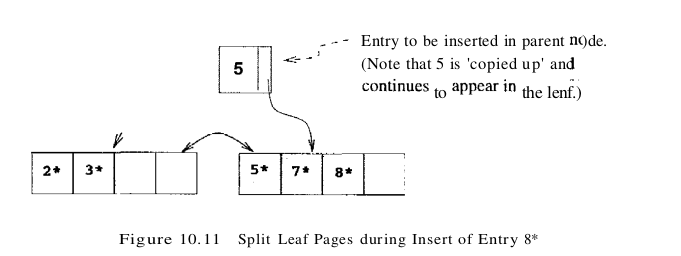
To illustrate insertion, let us continue with the sample tree shown in Figure 10.9. If we insert entry 8*, it belongs in the left-most leaf, which is already full. This insertion causes a split of the leaf page; the split pages are shown in Figure 10.11. The tree must now be adjusted to take the new leaf page into account, so we insert an entry consisting of the pair (5, pointer to new page) into the parent node. Note how the key 5, which discriminates between the split leaf page and its newly created sibling, is ‘copied up.’ We cannot just ‘push up’ 5, because every data entry must appear in a leaf page.
Since the parent node is also full, another split occurs. In general we have to split a non-leaf node when it is full, containing 2d keys and 2d + 1 pointers, and we have to add another index entry to account for a child split. We now have 2d+ 1 keys and 2d+2 pointers, yielding two minimally full non-leaf nodes, each containing d keys and d + 1 pointers, and an extra key, which we choose to be the ‘middle’ key. This key and a pointer to the second non-leaf node constitute an index entry that must be inserted into the parent of the split non-leaf node. The middle key is thus ‘pushed up’ the tree, in contrast to the case for a split of a leaf page.
The split pages in our example are shown in Figure 10.12. The index entry pointing to the new non-leaf node is the pair (17, pointer to new index-level page); note that the key value 17 is ‘pushed up’ the tree, in contrast to the splitting key value 5 in the leaf split, which was ‘copied up.’
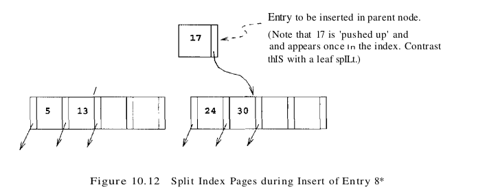
The difference in handling leaf-level and index-level splits arises from the B+ tree requirement that all data entries k* must reside in the leaves. This requirement prevents us from ‘pushing up’ 5 and leads to the slight redundancy of having some key values appearing in the leaf level as well as in some index level. However, range queries can be efficiently answered by just retrieving the sequence of leaf pages; the redundancy is a small price to pay for efficiency. In dealing with the index levels, we have more flexibility, and we ‘push up’ 17 to avoid having two copies of 17 in the index levels. Now, since the split node was the old root, we need to create a new root node to hold the entry that distinguishes the two split index pages. The tree after completing the insertion of the entry 8* is shown in Figure 10.13.

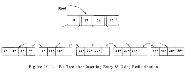
One variation of the insert algorithm tries to redistribute entries of a node N with a sibling before splitting the node; this improves average occupancy. The sibling of a node N, in this context, is a node that is immediately to the left or right of N and has the same parent as N.
To illustrate redistribution, reconsider insertion of entry 8* into the tree shown in Figure 10.9. The entry belongs in the left-most leaf, which is full. However, the (only) sibling of this leaf node contains only two entries and can thus accommodate more entries. We can therefore handle the insertion of 8* with a redistribution. Note how the entry in the parent node that points to the second leaf has a new key value; we ‘copy up’ the new low key value on the second leaf. This process is illustrated in Figure 10.14.
To determine whether redistribution is possible, we have to retrieve the sibling. If the sibling happens to be full, we have to split the node anyway. On average, checking whether redistribution is possible increases I/O for index node splits, especially if we check both siblings. (Checking whether redistribution is possible may reduce I/O if the redistribution succeeds whereas a split propagates up the tree, but this case is very infrequent.) If the file is growing, average occupancy will probably not be affected much even if we do not redistribute. Taking these considerations into account, not redistributing entries at non-leaf levels usually pays off.
If a split occurs at the leaf level, however, we have to retrieve a neighbor to adjust the previous and next-neighbor pointers with respect to the newly created leaf node. Therefore, a limited form of redistribution makes sense: If a leaf node is full, fetch a neighbor node; if it has space and has the same parent, redistribute the entries. Othenwise (the neighbor has diflerent parent, e.g., it is not a sibling, or it is also full) split the leaf node and adjust the previous and next-neighbor pointers in the split node, the newly created neighbor, and the old neighbor.
Delete
The algorithm for deletion takes an entry, finds the leaf node where it belongs, and deletes it. Pseudocode for the B+ tree deletion algorithm is given in Figure 10.15. The basic idea behind the algorithm is that we recursively delete the entry by calling the delete algorithm on the appropriate child node. We usually go down to the leaf node where the entry belongs, remove the entry from there, and return all the way back to the root node. Occasionally a node is at minimum occupancy before the deletion, and the deletion causes it to go below the occupancy threshold. When this happens, we must either redistribute entries from an adjacent sibling or merge the node with a sibling to maintain minimum occupancy. If entries are redistributed between two nodes, their parent node must be updated to reflect this; the key value in the index entry pointing to the second node must be changed to be the lowest search key in the second node. If two nodes are merged, their parent must be updated to reflect this by deleting the index entry for the second node; this index entry is pointed to by the pointer variable oldchildentry when the delete call returns to the parent node. If the last entry in the root node is deleted in this manner because one of its children was deleted, the height of the tree decreases by 1.

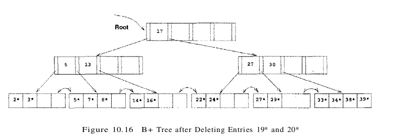
To illustrate deletion, let us consider the sample tree shown in Figure 10.13. To delete entry 19*, we simply remove it from the leaf page on which it appears, and we are done because the leaf still contains two entries. If we subsequently delete 20*, however, the leaf contains only one entry after the deletion. The (only) sibling of the leaf node that contained 20* has three entries, and we can therefore deal with the situation by redistribution; we move entry 24* to the leaf page that contained 20* and copy up the new splitting key (27, which is the new low key value of the leaf from which we borrowed 24*) into the parent. This process is illustrated in Figure 10.16.
Suppose that we now delete entry 24*. The affected leaf contains only one entry (22*) after the deletion, and the (only) sibling contains just two entries (27* and 29*). Therefore, we cannot redistribute entries. However, these two leaf nodes together contain only three entries and can be merged. While merging, we can ‘toss’ the entry ((27, pointer to second leaf page)) in the parent, which pointed to the second leaf page, because the second leaf page is empty after the merge and can be discarded. The right subtree of Figure 10.16 after this step in the deletion of entry 24* is shown in Figure 10.17.
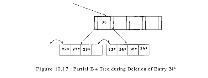
Deleting the entry (27, pointer to second leaf page) has created a non-leaf-level page with just one entry, which is below the minimum of d = 2. To fix this problem, we must either redistribute or merge. In either case, we must fetch a sibling. The only sibling of this node contains just two entries (with key values 5 and 13), and so redistribution is not possible; we must therefore merge.
The situation when we have to merge two non-leaf nodes is exactly the opposite of the situation when we have to split a non-leaf node. We have to split a non-leaf node when it contains 2d keys and 2d + 1 pointers, and we have to add another key pointer pair. Since we resort to merging two non-leaf nodes only when we cannot redistribute entries between them, the two nodes must be minimally full; that is, each must contain d keys and d + 1 pointers prior to the deletion. After merging the two nodes and removing the key pointer pair to be deleted, we have 2d - 1 keys and 2d + 1 pointers: Intuitively, the left-most pointer on the second merged node lacks a key value. To see what key value must be combined with this pointer to create a complete index entry, consider the parent of the two nodes being merged. The index entry pointing to one of the merged nodes must be deleted from the parent because the node is about to be discarded. The key value in this index entry is precisely the key value we need to complete the new merged node: The entries in the first node being merged, followed by the splitting key value that is ‘pulled down’ from the parent, followed by the entries in the second non-leaf node gives us a total of 2d keys and 2d + 1 pointers, which is a full non-leaf node. Note how the splitting key value in the parent is pulled down, in contrast to the case of merging two leaf nodes.
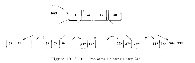
Consider the merging of two non-leaf nodes in our example. Together, the non-leaf node and the sibling to be merged contain only three entries, and they have a total of five pointers to leaf nodes. To merge the two nodes, we also need to pull down the index entry in their parent that currently discriminates between these nodes. This index entry has key value 17, and so we create a new entry (17, left-most child pointer in sibling). Now we have a total of four entries and five child pointers, which can fit on one page in a tree of order d = 2. Note that pulling down the splitting key 17 means that it will no longer appear in the parent node following the merge. After we merge the affected non-leaf node and its sibling by putting all the entries on one page and discarding the empty sibling page, the new node is the only child of the old root, which can therefore be discarded. The tree after completing all these steps in the deletion of entry 24* is shown in Figure 10.18.
The previous examples illustrated redistribution of entries across leaves and merging of both leaf-level and non-leaf-level pages. The remaining case is that of redistribution of entries between non-leaf-level pages. To understand this case, consider the intermediate right subtree shown in Figure 10.17. We would arrive at the same intermediate right subtree if we try to delete 24* from a tree similar to the one shown in Figure 10.16 but with the left subtree and root key value as shown in Figure 10.19. The tree in Figure 10.19 illustrates an intermediate stage during the deletion of 24*. (Try to construct the initial tree. )
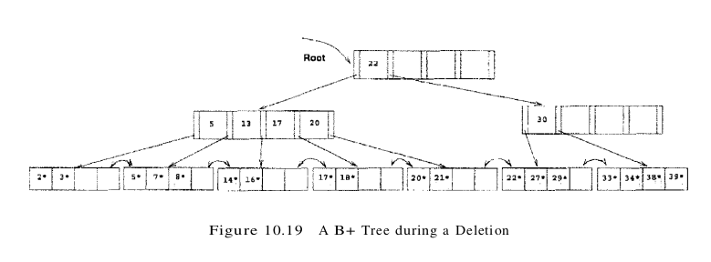
In contrast to the case when we deleted 24* from the tree of Figure 10.16, the non-leaf level node containing key value 30 now has a sibling that can spare entries (the entries with key values 17 and 20). We move these entries over from the sibling. Note that, in doing so, we essentially push them through the splitting entry in their parent node (the root), which takes care of the fact that 17 becomes the new low key value on the right and therefore must replace the old splitting key in the root (the key value 22). The tree with all these changes is shown in Figure 10.20.

In concluding our discussion of deletion, we note that we retrieve only one sibling of a node. If this node has spare entries, we use redistribution; otherwise, we merge. If the node has a second sibling, it may be worth retrieving that sibling as well to check for the possibility of redistribution. Chances are high that redistribution is possible, and unlike merging, redistribution is guaranteed to propagate no further than the parent node. Also, the pages have more space on them, which reduces the likelihood of a split on subsequent insertions. (Remember, files typically grow, not shrink!) However, the number of times that this case arises (the node becomes less than half-full and the first sibling cannot spare an entry) is not very high, so it is not essential to implement this refinement of the basic algorithm that we presented.
Duplicates
The search, insertion, and deletion algorithms that we presented ignore the issue of duplicate keys, that is, several data entries with the same key value. We now discuss how duplicates can be handled.
The basic search algorithm assumes that all entries with a given key value reside on a single leaf page. One way to satisfy this assumption is to use overflow pages to deal with duplicates. (In ISAM, of course, we have overflow pages in any case, and duplicates are easily handled.) Typically, however, we use an alternative approach for duplicates. We handle them just like any other entries and several leaf pages may contain entries with a given key value. To retrieve all data entries with a given key value, we must search for the left-most data entry with the given key value and then possibly retrieve more than one leaf page (using the leaf sequence pointers). Modifying the search algorithm to find the left-most data entry in an index with duplicates is an interesting exercise.
One problem with this approach is that, when a record is deleted, if we use Alternative (2) for data entries, finding the corresponding data entry to delete in the B+ tree index could be inefficient because we may have to check several duplicate entries (key, rid) with the same key value. This problem can be addressed by considering the rid value in the data entry to be part of the search key, for purposes of positioning the data entry in the tree. This solution effectively turns the index into a unique index (i.e” no duplicates), Remember that a search key can be any sequence of fields in this variant, the rid of the data record is essentially treated as another field while constructing the search key.
Alternative (3) for data entries leads to a natural solution for duplicates, but if we have a large number of duplicates, a single data entry could span multiple pages. And of course, when a data record is deleted, finding the rid to delete from the corresponding data entry can be inefficient, The solution to this problem is similar to the one discussed previously for Alternative (2): We can maintain the list of rids within each data entry in sorted order (say, by page number and then slot number if a rid consists of a page id and a slot id).
B+ Trees in Practice
Key Compression
The height of a B+ tree depends on the number of data entries and the size of index entries. The size of index entries determines the number of index entries that will fit on a page and, therefore, the fan-out of the tree. Since the height of the tree is proportional to $log_{2} fan-out$ of data entries, and the number of disk I/Os to retrieve a data entry is equal to the height (unless some pages are found in the buffer pool), it is clearly important to maximize the fan-out to minimize the height.
An index entry contains a search key value and a page pointer. Hence the size depends primarily on the size of the search key value. If search key values are very long (for instance, the name Devarakonda Venkataramana Sathyanarayana Seshasayee Yellamanchali Murthy, or Donaudampfschifffahrts-kapitansanwiirtersmiitze), not many index entries will fit on a page: Fan-out is low, and the height of the tree is large.
On the other hand, search key values in index entries are used only to direct traffic to the appropriate leaf. When we want to locate data entries with a given search key value, we compare this search key value with the search key values of index entries (on a path from the root to the desired leaf). During the comparison at an index-level node, we want to identify two index entries with search key values $k_1 $ and $k_2$ such that the desired search key value k falls between $k_1 $ and $k_2$. To accomplish this, we need not store search key values in their entirety in index entries.
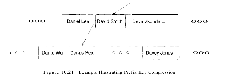
For example, suppose we have two adjacent index entries in a node, with search key values ‘David Smith’ and ‘Devarakonda … ‘ To discriminate between these two values, it is sufficient to store the abbreviated forms ‘Da’ and ‘De.’ More generally, the meaning of the entry ‘David Smith’ in the B+ tree is that every value in the subtree pointed to by the pointer to the left of ‘David Smith’ is less than ‘David Smith,’ and every value in the subtree pointed to by the pointer to the right of ‘David Smith’ is (greater than or equal to ‘David Smith’ and) less than ‘Devarakonda … ‘
To ensure such semantics for an entry is preserved, while compressing the entry with key ‘David Smith,’ we must examine the largest key value in the subtree to the left of ‘David Smith’ and the smallest key value in the subtree to the right of ‘David Smith,’ not just the index entries (‘Daniel Lee’ and ‘Devarakonda … ‘) that are its neighbors. This point is illustrated in Figure 10.21; the value ‘Davey Jones’ is greater than ‘Dav,’ and thus, ‘David Smith’ can be abbreviated only to ‘Davi,’ not to ‘Dav.’
This technique. called prefix key compression or simply key compression, is supported in many commercial implementations of B+ trees. It can substantially increase the fan-out of a tree. We do not discuss the details of the insertion and deletion algorithms in the presence of key compression.
Bulk-Loading a B+ Tree
Entries are added to a B+ tree in two ways. First, we may have an existing collection of data records with a B+ tree index on it; whenever a record is added to the collection, a corresponding entry must be added to the B+ tree as well. (Of course, a similar comment applies to deletions.) Second, we may have a collection of data records for which we want to create a B+ tree index on some key field(s). In this situation, we can start with an empty tree and insert an entry for each data record, one at a time, using the standard insertion algorithm. However, this approach is likely to be quite expensive because each entry requires us to start from the root and go down to the appropriate leaf page. Even though the index-level pages are likely to stay in the buffer pool between successive requests, the overhead is still considerable.
For this reason many systems provide a bulk-loading utility for creating a B+ tree index on an existing collection of data records. The first step is to sort the data entries k* to be inserted into the (to be created) B+ tree according to the search key k. (If the entries are key-pointer pairs, sorting them does not mean sorting the data records that are pointed to, of course.) We use a running example to illustrate the bulk-loading algorithm. We assume that each data page can hold only two entries, and that each index page can hold two entries and an additional pointer (i.e., the B+ tree is assumed to be of order d = 1).
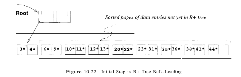
After the data entries have been sorted, we allocate an empty page to serve as the root and insert a pointer to the first page of (sorted) entries into it. We illustrate this process in Figure 10.22, using a sample set of nine sorted pages of data entries.
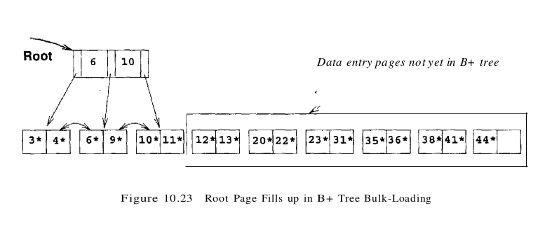
We then add one entry to the root page for each page of the sorted data entries. The new entry consists of (low key value on page, pointer to page). We proceed until the root page is full; see Figure 10.23. To insert the entry for the next page of data entries, we must split the root and create a new root page. We show this step in Figure 10.24.
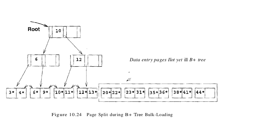
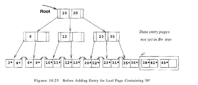
We have redistributed the entries evenly between the two children of the root, in anticipation of the fact that the B+ tree is likely to grow. Although it is difficult to illustrate these options when at most two entries fit on a page, we could also have just left all the entries on the old page or filled up some desired fraction of that page (say, 80 percent). These alternatives are simple variants of the basic idea. To continue with the bulk-loading example, entries for the leaf pages are always inserted into the right-most index page just above the leaf level. When the right-most index page above the leaf level fills up, it is split. This action may cause a split of the right-most index page one step closer to the root, as illustrated in Figures 10.25 and 10.26.

Note that splits occur only on the right-most path from the root to the leaf level. Let us consider the cost of creating an index on an existing collection of records. This operation consists of three steps: (1) creating the data entries to insert in the index, (2) sorting the data entries, and (3) building the index from the sorted entries. The first step involves scanning the records and writing out the corresponding data entries; the cost is (R + E) I/Os, where R is the number of pages containing records and E is the number of pages containing data entries. you will see that the index entries can be generated in sorted order at a cost of about 3E I/Os. These entries can then be inserted into the index as they are generated, using the bulk-loading algorithm discussed in this section. The cost of the third step, that is, inserting the entries into the index, is then just the cost of writing out all index pages.
The Order Concept
We presented B+ trees using the parameter d to denote minimum occupancy. It is worth noting that the concept of order (i.e., the parameter d), while useful for teaching B+ tree concepts, must usually be relaxed in practice and replaced by a physical space criterion; for example, that nodes must be kept at least half-full. One reason for this is that leaf nodes and non-leaf nodes can usually hold different numbers of entries. Recall that B+ tree nodes are disk pages and non-leaf nodes contain only search keys and node pointers, while leaf nodes can contain the actual data records. Obviously, the size of a data record is likely to be quite a bit larger than the size of a search entry, so many more search entries than records fit on a disk page. A second reason for relaxing the order concept is that the search key may contain a character string field (e.g., the name field of Students) whose size varies from record to record; such a search key leads to variable-size data entries and index entries, and the number of entries that will fit on a disk page becomes variable. Finally, even if the index is built on a fixed-size field, several records may still have the same search key value (e.g., several Students records may have the same gpa or name value). This situation can also lead to variable-size leaf entries (if we use Alternative (3) for data entries). Because of all these complications, the concept of order is typically replaced by a simple physical criterion (e.g., merge if possible when more than half of the space in the node is unused).
The Effect of Inserts and Deletes on Rids
If the leaf pages contain data records – that is, the B+ tree is a clustered index – then operations such as splits, merges, and redistributions can change rids. Recall that a typical representation for a rid is some combination of (physical) page number and slot number. This scheme allows us to move records within a page if an appropriate page format is chosen but not across pages, as is the case with operations such as splits. So unless rids are chosen to be independent of page numbers, an operation such as split or merge in a clustered B+ tree may require compensating updates to other indexes on the same data. A similar comment holds for any dynamic clustered index, regardless of whether it is tree-based or hash-based. Of course, the problem does not arise with nonclustered indexes, because only index entries are moved around.