#8 Storing Data: Disks and Files

• Magnetic Disks
• Redundant Arrays of Independent Disks
  • Data Striping
  • Redundancy
  • Levels of Redundancy
• Disk Space Management
• Buffer Manager
  • Buffer Replacement Policies
  • Buffer Management in DBMS versus OS
• Files of Records
  • Implementing Heap Files
• Page Formats
• Record Formats

Memory in a computer system is arranged in a hierarchy. At the top, we have primary storage, which consists of cache and main memory and provides very fast access to data. Then comes secondary storage, which consists of slower devices, such as magnetic disks. Tertiary storage is the slowest class of storage devices; for example, optical disks and tapes. Currently, the cost of a given amount of main memory is about 100 times the cost of the same amount of disk space, and tapes are even less expensive than disks. Slower storage devices such as tapes and disks play an important role in database systems because the amount of data is typically very large. Since buying enough main memory to store all data is prohibitively expensive, we must store data on tapes and disks and build database systems that can retrieve data from lower levels of the memory hierarchy into main mernory as needed for processing.

There are reasons other than cost for storing data on secondary and tertiary storage. On systems with 32-bit addressing, only $2^{32}$ bytes can be directly referenced in main memory; the number of data objects may exceed this number. Further, data must be maintained across program executions. This requires storage devices that retain information when the computer is restarted (after a shutdown or a crash); we call such storage nonvolatile. Primary storage is usually volatile (although it is possible to make it nonvolatile by adding a battery backup feature), whereas secondary and tertiary storage are nonvolatile.

Magnetic Disks

A DBMS provides seamless access to data on disk; applications need not worry about whether data is in main memory or disk. To understand how disks work, eonsider Figure 9.2, which shows the structure of a disk in simplified form.

Data is stored on disk in units called disk blocks. A disk block is a contiguous sequence of bytes and is the unit in which data is written to a disk and read from a disk. Blocks are arranged in concentric rings called tracks, on one or more platters. Tracks can be recorded on one or both surfaces of a platter; we refer to platters as single-sided or double-sided, accordingly. The set of all tracks with the same diameter is called a cylinder, because the space occupied by these tracks is shaped like a cylinder; a cylinder contains one track per platter surface. Each track is divided into arcs, called sectors, whose size is a characteristic of the disk and cannot be changed. The size of a disk block can be set when the disk is initialized as a multiple of the sector size.

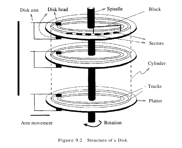
An array of disk heads, one per recorded surface, is moved as a unit; when one head is positioned over a block, the other heads are in identical positions with respect to their platters. To read or write a block, a disk head must be positioned on top of the block.

Current systems typically allow at most one disk head to read or write at any one time. All the disk heads cannot read or write in parallel -this technique would increase data transfer rates by a factor equal to the number of disk heads and considerably speed up sequential scans. The reason they cannot is that it is very difficult to ensure that all the heads are perfectly aligned on the corresponding tracks. Current approaches are both expensive and more prone to faults than disks with a single active head. In practice, very few commercial products support this capability and then only in a limited way; for example, two disk heads may be able to operate in parallel.

A disk controller interfaces a disk drive to the computer. It implements commands to read or write a sector by moving the arm assembly and transferring data to and from the disk surfaces. A checksum is computed for when data is written to a sector and stored with the sector. The checksum is computed again when the data on the sector is read back. If the sector is corrupted or the read is faulty for some reason, it is very unlikely that the checksum computed when the sector is read matches the checksum computed when the sector was written. The controller computes checksums, and if it detects an error, it tries to read the sector again. (Of course, it signals a failure if the sector is corrupted and read fails repeatedly.)

While direct access to any desired location in main memory takes approximately the same time, determining the time to access a location on disk is more complicated. The time to access a disk block has several components. Seek time is the time taken to move the disk heads to the track on which a desired block is located. As the size of a platter decreases, seek times also decrease, since we have to move a disk head a shorter distance. Typical platter diameters are 3.5 inches and 5.25 inches. Rotational delay is the waiting time for the desired block to rotate under the disk head; it is the time required for half a rotation all average and is usually less than seek time. Transfer time is the time to actually read or write the data in the block once the head is positioned, that is, the time for the disk to rotate over the block.

1. Data must be in memory for the DBMS to operate on it.
2. The unit for data transfer between disk and main memory is a block; if a single item on a block is needed, the entire block is transferred. Reading or writing a disk block is called an I/O (for input/output) operation.
3. The time to read or write a block varies, depending on the location of the data: access time = seek time + rotational delay + transfer time

These observations imply that the time taken for database operations is affected significantly by how data is stored on disks. The time for moving blocks to or from disk usually dominates the time taken for database operations. To minimize this time, it is necessary to locate data records strategically on disk because of the geometry and mechanics of disks. In essence, if two records are frequently used together, we should place them close together. The ‘closest’ that two records can be on a disk is to be on the same block. In decreasing order of closeness, they could be on the same track, the same cylinder, or an adjacent cylinder.

Two records on the same block are obviously as close together as possible, because they are read or written as part of the same block. As the platter spins, other blocks on the track being read or written rotate under the active head. In current disk designs, all the data on a track can be read or written in one revolution. After a track is read or written, another disk head becomes active, and another track in the same cylinder is read or written. This process continues until all tracks in the current cylinder are read or written, and then the arm assembly moves (in or out) to an adjacent cylinder. Thus, we have a natural notion of ‘closeness’ for blocks, which we can extend to a notion of next and previous blocks. Exploiting this notion of next by arranging records so they are read or written sequentially is very important in reducing the time spent in disk I/Os. Sequential access minimizes seek time and rotational delay and is much faster than random access.

Redundant Arrays of Independent Disks

Disks are potential bottlenecks for system performance and storage system reliability. Even though disk performance has been improving continuously, microprocessor performance has advanced much more rapidly. The performance of microprocessors has improved at about 50 percent or more per year, but disk access times have improved at a rate of about 10 percent per year and disk transfer rates at a rate of about 20 percent per year. In addition, since disks contain mechanical elements, they have much higher failure rates than electronic parts of a computer system. If a disk fails, all the data stored on it is lost.

A disk array is an arrangement of several disks, organized to increase performance and improve reliability of the resulting storage system. Performance is increased through data striping. Data striping distributes data over several disks to give the impression of having a single large, very fast disk. Reliability is improved through redundancy. Instead of having a single copy of the data, redundant information is maintained. The redundant information is carefully organized so that, in case of a disk failure, it can be used to reconstruct the contents of the failed disk. Disk arrays that implement a combination of data striping and redundancy are called redundant arrays of independent disks, or in short, RAID. Several RAID organizations, referred to as RAID levels, have been proposed. Each RAID level represents a different trade-off between reliability and performance.

Data Striping

A disk array gives the user the abstraction of having a single, very large disk. If the user issues an I/O request, we first identify the set of physical disk blocks that store the data requested. These disk blocks may reside on a single disk in the array or may be distributed over several disks in the array. Then the set of blocks is retrieved from the disk(s) involved. Thus, how we distribute the data over the disks in the array influences how many disks are involved when an I/O request is processed.

In data striping, the data is segmented into equal-size partitions distributed over multiple disks. The size of the partition is called the striping unit. The partition are usually distributed using a round-robin algorithm: If the disk array consists of D disks, then partition i is written onto disk i mod D.

As an example, consider a striping unit of one bit. Since any D successive data bits are spread over all D data disks in the array, all I/O requests involve D disks in the array. Since the smallest unit of transfer from a disk is a block, each I/O request involves transfer of at least D blocks. Since we can read the D blocks from the D disks in parallel, the transfer rate of each request is D times the transfer rate of a single disk; each request uses the aggregated bandwidth of all disks in the array. But the disk access time of the array is basically the access time of a single disk, since all disk heads have to move for all requests. Therefore, for a disk array with a striping unit of a single bit, the number of requests per time unit that the array can process and the average response time for each individual request are similar to that of a single disk.

As another example, consider a striping unit of a disk block. In this case, I/O requests of the size of a disk block are processed by one disk in the array. If many I/O requests of the size of a disk block are made, and the requested blocks reside on different disks, we can process all requests in parallel and thus reduce the average response time of an I/O request. Since we distributed the striping partitions round-robin, large requests of the size of many contiguous blocks involve all disks. We can process the request by all disks in parallel and thus increase the transfer rate to the aggregated bandwidth of all D disks.

Redundancy

While having more disks increases storage system performance, it also lowers overall storage system reliability. Assume that the mean-time-to-failure (MTTF), of a single disk is 50, 000 hours (about 5.7 years). Then, the MTTF of an array of 100 disks is only 50, 000/100 = 500 hours or about 21 days, assuming that failures occur independently and the failure probability of a disk does not change over time. (Actually, disks have a higher failure probability early and late in their lifetimes. Early failures are often due to undetected manufacturing defects; late failures occur since the disk wears out. Failures do not occur independently either: consider a fire in the building, an earthquake, or purchase of a set of disks that come from a ‘bad’ manufacturing batch.)

Reliability of a disk array can be increased by storing redundant information. If a disk fails, the redundant information is used to reconstruct the data on the failed disk. Redundancy can immensely increase the MTTF of a disk array. When incorporating redundancy into a disk array design, we have to make two choices. First, we have to decide where to store the redundant information. We can either store the redundant information on a small number of check disks or distribute the redundant information uniformly over all disks.

The second choice we have to make is how to compute the redundant information. Most disk arrays store parity information: In the parity scheme, an extra check disk contains information that can be used to recover from failure of anyone disk in the array. Assume that we have a disk array with D disks and consider the first bit on each data disk. Suppose that i of the D data bits are 1. The first bit on the check disk is set to 1 if i is odd; otherwise, it is set to O. This bit on the check disk is called the parity of the data bits. The check disk contains parity information for each set of corresponding D data bits.

To recover the value of the first bit of a failed disk we first count the number of bits that are 1 on the D - 1 nonfailed disks; let this number be j. If j is odd and the parity bit is 1, or if j is even and the parity bit is 0, then the value of the bit on the failed disk must have been 0. Otherwise, the value of the bit on the failed disk must have been 1. Thus, with parity we can recover from failure of anyone disk. Reconstruction of the lost information involves reading all data disks and the check disk. For example, with an additional 10 disks with redundant information, the MTTF of our example storage system with 100 data disks can be increased to more than 250 years. What is more important, a large MTTF implies a small failure probability during the actual usage time of the storage system, which is usually much smaller than the reported lifetime or the MTTF. (Who actually uses 10-year-old disks?)

In a RAID system, the disk array is partitioned into reliability groups, where a reliability group consists of a set of data disks and a set of check disks. A common redundancy scheme is applied to each group. The number of check disks depends on the RAID level chosen. In the remainder of this section, we assume for ease of explanation that there is only one reliability group. The reader should keep in mind that actual RAID implementations consist of several reliability groups, and the number of groups plays a role in the overall reliability of the resulting storage system.

Levels of Redundancy

Throughout the discussion of the different RAID levels, we consider sample data that would just fit on four disks. That is, with no RAID technology our storage system would consist of exactly four data disks. Depending on the RAID level chosen, the number of additional disb varies from zero to four.

• Level 0: Nonredundant. A RAID Level 0 system uses data striping to increase the maximum bandwidth available. No redundant information is maintained. While being the solution with the lowest cost, reliability is a problem, since the MTTF decreases linearly with the number of disk drives in the array. RAID Level 0 has the best write performance of all RAID levels, because absence of redundant information implies that no redundant information needs to be updated. Interestingly, RAID Level 0 does not have the best read perfonnancc of all RAID levels, since systems with redundancy have a choice of scheduling disk accesses. In our example, the RAID Level 0 solution consists of only four data disks. Independent of the number of data disks, the effective space utilization for a RAID Level 0 system is always 100 percent.
• Level 1: Mirrored. A RAID Level 1 system is the most expensive solution. Instead of having one copy of the data, two identical copies of the data on two different disks are maintained. This type of redundancy is often called mirroring. Every write of a disk block involves a write on both disks. These writes may not be performed simultaneously, since a global system failure (e.g., due to a power outage) could occur while writing the blocks and then leave both copies in an inconsistent state. Therefore, we always write a block on one disk first and then write the other copy on the mirror disk. Since two copies of each block exist on different disks, we can distribute reads between the two disks and allow parallel reads of different disk blocks that conceptually reside on the same disk. A read of a block can be scheduled to the disk that has the smaller expected access time. RAID Level 1 does not stripe the data over different disks, so the transfer rate for a single request is comparable to the transfer rate of a single disk. In our example, we need four data and four check disks with mirrored data for a RAID Levell implementation. The effective space utilization is 50 percent, independent of the number of data disks.
• Level 0 + 1: Striping and Mirroring. RAID Level 0+ 1 - sometimes also referred to as RAID Level 10 - combines striping and mirroring. As in RAID Level 1 read requests of the size of a disk block can be scheduled both to a disk and its mirror image. In addition, read requests of the size of several contiguous blocks benefit from the aggregated bandwidth of all disks. Thc cost for writes is analogous to RAID Level 1. As in RAID Level 1, our example with four data disks requires four check disks and the effective space utilization is always 50 percent.
• Level 2: Error-Correcting Codes. In RAID Level 2, the striping unit is a single bit. The redundancy scheme used is Hamming code. In our example with four data disks, only three check disks are needed. In general, the number of check disks grows logarithmically with the number of data disks. Striping at the bit level has the implication that in a disk array with D data disks, the smallest unit of transfer for a read is a set of D blocks. Therefore, Level 2 is good for workloads with many large requests, since for each request, the aggregated bandwidth of all data disks is used. But RAID Level 2 is bad for small requests of the size of an individual block for the same reason. A write of a block involves reading D blocks into main memory, modifying D + C blocks, and writing D + C blocks to disk, where C is the number of check disks. This sequence of steps is called a read-modify-write cycle. For a RAID Level 2 implementation with four data disks, three check disks are needed. In our example, the effective space utilization is about 57 percent. The effective space utilization increases with the number of data disks. For example, in a setup with 10 data disks, four check disks are needed and the effective space utilization is 71 percent. In a setup with 25 data disks, five check disks are required and the effective space utilization grows to 83 percent.
• Level 3: Bit-Interleaved Parity. While the redundancy scheme used in RAID Level 2 improves in terms of cost over RAID Level 1, it keeps more redundant information than is necessary. Hamming code, as used in RAID Level 2, has the advantage of being able to identify which disk has failed. But disk controllers can easily detect which disk has failed. Therefore, the check disks do not need to contain information to identify the failed disk. Information to recover the lost data is sufficient. Instead of using several disks to store Hamming code, RAID Level 3 has a single check disk with parity information. Thus, the reliability overhead for RAID Level 3 is a single disk, the lowest overhead possible. The performance characteristics of RAID Levels 2 and 3 are very similar. RAID Level 3 can also process only one I/O at a time, the minimum transfer unit is D blocks, and a write requires a read-modify-write cycle.
• Level 4: Block-Interleaved Parity. RAID Level 4 has a striping unit of a disk block, instead of a single bit as in RAID Level 3. Block-level striping has the advantage that read requests of the size of a disk block can be served entirely by the disk where the requested block resides. Large read requests of several disk blocks can still utilize the aggregated bandwidth of the D disks. The write of a single block still requires a read-modify-write cycle, but only one data disk and the check disk are involved. The parity on the check disk can be updated without reading all D disk blocks, because the new parity can be obtained by noticing the differences between the old data block and the new data block and then applying the difference to the parity block on the check disk: NewParity = (OldData XOR NewData) XOR OldParity. The read-modify-write cycle involves reading of the old data block and the old parity block, modifying the two blocks, and writing them back to disk, resulting in four disk accesses per write. Since the check disk is involved in each write, it can easily become the bottleneck. RAID Level 3 and 4 configurations with four data disks require just a single check disk. In our example, the effective space utilization is 80 percent. The effective space utilization increases with the number of data disks, since always only one check disk is necessary.
• Level 5: Block-Interleaved Distributed Parity. RAID Level 5 improves on Level 4 by distributing the parity blocks uniformly over all disks, instead of storing them on a single check disk. This distribution has two advantages. First, several write requests could be processed in parallel, since the bottleneck of a unique check disk has been eliminated. Second, read requests have a higher level of parallelism. Since the data is distributed over all disks, read requests involve all disks, whereas in systems with a dedicated check disk the check disk never participates in reads. A RAID Level 5 system has the best performance of all RAID levels with redundancy for small and large read and large write requests. Small writes still require a read-modify-write cycle and are thus less efficient than in RAID Level 1. In our example, the corresponding RAID Level 5 system has five disks overall and thus the effective space utilization is the same as in RAID Levels 3 and 4.
• Level 6: P + Q Redundancy. The motivation for RAID Level 6 is the observation that recovery from failure of a single disk is not sufficient in very large disk arrays. First, in large disk arrays, a second disk might fail before replacement of an already failed disk could take place. In addition, the probability of a disk failure during recovery of a failed disk is not negligible. A RAID Level 6 system uses Reed-Solomon codes to be able to recover from up to two simultaneous disk failures. RAID Level 6 requires (conceptually) two check disks, but it also uniformly distributes redundant information at the block level as in RAID Level 5. Thus. the performance characteristics for small and large read requests and for large write requests are analogous to RAID Level 5. For small writes, the read-modify-write procedure involves six instead of four disks as compared to RAID Level 5, since two blocks with redundant information need to be updated. For a RAID Level 6 system with storage capacity equal to four data disks, six disks are required. In our example, the effective space utilization is 66 percent.

If data loss is not an issue, RAID Level 0 improves overall system performance at the lowest cost. RAID Level 0 + 1 is superior to RAID Level 1. The main application areas for RAID Level 0 + 1 systems are small storage subsystems where the cost of mirroring is moderate. Sometimes, RAID Level 0 + 1 is used for applications that have a high percentage of writes in their workload, since RAID Level 0 + 1 provides the best write performance. RAID Levels 2 and 4 are always inferior to RAID Levels 3 and 5, respectively. RAID Level 3 is appropriate for workloads consisting mainly of large transfer requests of several contiguous blocks. The performance of a RAID Level 3 system is bad for workloads with many small requests of a single disk block. RAID Level 5 is a good general-purpose solution. It provides high performance for large as well as small requests. RAID Level 6 is appropriate if a higher level of reliability is required.

Disk Space Management

The lowest level of software in the DBMS architecture, called the disk space manager, manages space on disk. Abstractly, the disk space manager supports the concept of a page as a unit of data and provides commands to allocate or deallocate a page and read or write a page. The size of a page is chosen to be the size of a disk block and pages are stored as disk blocks so that reading or writing a page can be done in one disk I/O. It is often useful to allocate a sequence of pages as a contiguous sequence of blocks to hold data frequently accessed in sequential order. This capability is essential for exploiting the advantages of sequentially accessing disk blocks. Such a capability, if desired, must be provided by the disk space manager to higher-level layers of the DBMS.

A database grows and shrinks as records are inserted and deleted over time. The disk space manager keeps track of which disk blocks are in use, in addition to keeping track of which pages are on which disk blocks. Although it is likely that blocks are initially allocated sequentially on disk, subsequent allocations and deallocations could in general create ‘holes.’ One way to keep track of block usage is to maintain a list of free blocks. As blocks are deallocated (by the higher-level software that requests and uses these blocks), we can add them to the free list for future use. A pointer to the first block on the free block list is stored in a known location on disk. A second way is to maintain a bitmap with one bit for each disk block, which indicates whether a block is in use or not. A bitmap also allows very fast identification and allocation of contiguous areas on disk. This is difficult to accomplish with a linked list approach.

Operating systems also manage space on disk. Typically, an operating system supports the abstraction of a file as a sequence of bytes. The as manages space on the disk and translates requests, such as “Read byte i of file f,” into corresponding low-level instructions: “Read block m of track t of cylinder c of disk d.” A database disk space manager could be built using OS files. For example, the entire database could reside in one or more files for which a number of blocks are allocated (by the OS) and initialized. The disk space manager is then responsible for managing the space in these OS files. Many database systems do not rely on the OS file system and instead do their own disk management, either from scratch or by extending facilities. The reasons are practical as well as technical. One practical reason is that a DBMS vendor who wishes to support several as platforms cannot assume features specific to any OS, for portability, and would therefore try to make the DBMS code as self-contained as possible. A technical reason is that on a 32-bit systern, the largest file size is 4 GB, whereas a DBMS may want to access a single file larger than that. A related problem is that files cannot span disk devices, which is often desirable or even necessary in a DBMS.

Buffer Manager

To understand the role of the buffer manager, consider a simple example. Suppose that the database contains 1 million pages, but only 1000 pages of main memory are available for holding data. Consider a query that requires a scan of the entire file. Because all the data cannot be brought into main memory at one time, the DBMS must bring pages into main memory as they are needed and, in the process, decide what existing page in main memory to replace to make space for the new page. The policy used to decide which page to replace is called the replacement policy.

The buffer manager is the software layer responsible for bringing pages from disk to main memory as needed. The buffer manager manages the available main memory by partitioning it into a collection of pages, which we collectively refer to as the buffer pool. The main memory pages in the buffer pool are called frames; it is convenient to think of them as slots that can hold a page (which usually resides on disk or other secondary storage media). Higher levels of the DBMS code can be written without worrying about whether data pages are in memory or not; they ask the buffer manager for the page, and it is brought into a frame in the buffer pool if it is not already there. Of course, the higher-level code that requests a page must also release the page when it is no longer needed, by informing the buffer manager, so that the frame containing the page can be reused. The higher-level code must also inform the buffer manager if it modifies the requested page; the buffer manager then makes sure that the change is propagated to the copy of the page on disk. Buffer management is illustrated in Figure 9.3.

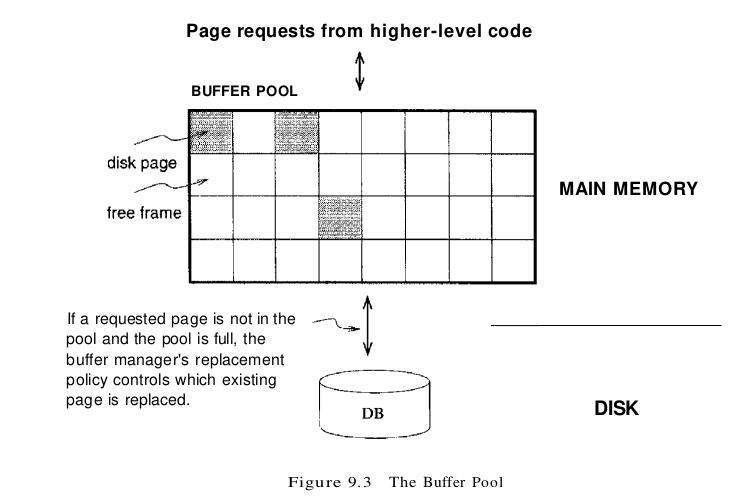
In addition to the buffer pool itself, the buffer manager maintains some bookkeeping information and two variables for each frame in the pool: pin_count and dirty. The number of times that the page currently in a given frame has been requested but not released-the number of current users of the page–is recorded in the pin_count variable for that frame. The Boolean variable dirty indicates whether the page has been modified since it was brought into the buffer pool from disk.

Initially, the pin_count for every frame is set to 0, and the dirty bits are turned off. When a page is requested the buffer manager does the following:

1. Checks the buffer pool to see if some frame contains the requested page and, if so, increments the pin_count of that frame. If the page is not in the pool, the buffer manager brings it in as follows:
   • Chooses a frame for replacement, using the replacement policy, and increments its pin_count.
   • If the dirty bit for the replacement frame is on, writes the page it contains to disk (that is, the disk copy of the page is overwritten with the contents of the frame).
   • Reads the requested page into the replacement frame.
2. Returns the (main memory) address of the frame containing the requested page to the requestor.

Incrementing pin_count is often called pinning the requested page in its frame. When the code that calls the buffer manager and requests the page subsequently calls the buffer manager and releases the page, the pin_count of the frame containing the requested page is decremented. This is called unpinning the page. If the requestor has modified the page, it also informs the buffer manager of this at the time that it unpins the page, and the dirty bit for the frame is set. The buffer manager will not read another page into a frame until its pin_count becomes 0, that is, until all requestors of the page have unpinned it. If a requested page is not in the buffer pool and a free frame is not available in the buffer pool, a frame with pin_count 0 is chosen for replacement. If there are many such frames, a frame is chosen according to the buffer manager’s replacement policy.

When a page is eventually chosen for replacement, if the dirty bit is not set, it means that the page has not been modified since being brought into main memory. Hence, there is no need to write the page back to disk; the copy on disk is identical to the copy in the frame, and the frame can simply be overwritten by the newly requested page. Otherwise, the modifications to the page must be propagated to the copy on disk. (The crash recovery protocol may impose further restrictions. For example, in the Write-Ahead Log (WAL) protocol, special log records are used to describe the changes made to a page. The log records pertaining to the page to be replaced may well be in the buffer; if so, the protocol requires that they be written to disk before the page is written to disk.) If no page in the buffer pool has pin_count 0 and a page that is not in the pool is requested, the buffer manager must wait until some page is released before responding to the page request. In practice, the transaction requesting the page may simply be aborted in this situation! So pages should be released–by the code that calls the buffer manager to request the page as soon as possible. A good question to ask at this point is, “What if a page is requested by several different transactions?” That is, what if the page is requested by programs executing independently on behalf of different users? Such programs could make conflicting changes to the page. The locking protocol (enforced by higher-level DBMS code, in particular the transaction manager) ensures that each transaction obtains a shared or exclusive lock before requesting a page to read or modify. Two different transactions cannot hold an exclusive lock on the same page at the same time; this is how conflicting changes are prevented. The buffer manager simply assumes that the appropriate lock has been obtained before a page is requested.

Buffer Replacement Policies

The best-known replacement policy is least recently used (LRU). This can be implemented in the buffer manager using a queue of pointers to frames with pin_count O. A frame is added to the end of the queue when it becomes a candidate for replacement (that is, when the pin_count goes to 0). The page chosen for replacement is the one in the frame at the head of the queue.

A variant of LRU, called clock replacement, has similar behavior but less overhead. The idea is to choose a page for replacement using a current variable that takes on values 1 through N, where N is the number of buffer frames, in circular order. We can think of the frames being arranged in a circle, like a clock’s face, and current as a clock hand moving across the face. To approximate LRU behavior, each frame also has an associated referenced bit, which is turned on when the page pin_count goes to O. The current frame is considered for replacement. If the frame is not chosen for replacement, current is incremented and the next frame is considered; this process is repeated until some frame is chosen. If the current frame has pin_count greater than 0, then it is not a candidate for replacement and current is incremented. If the current frame has the referenced bit turned on, the clock algorithm turns the referenced bit off and increments current–this way, a recently referenced page is less likely to be replaced. If the current frame has pin_count 0 and its referenced bit is off, then the page in it is chosen for replacement. If all frames are pinned in some sweep of the clock hand (that is, the value of current is incremented until it repeats), this means that no page in the buffer pool is a replacement candidate.

The LRU and clock policies are not always the best replacement strategies for a database system, particularly if many user requests require sequential scans of the data. Consider the following illustrative situation. Suppose the buffer pool has 10 frames, and the file to be scanned has 10 or fewer pages. Assuming, for simplicity, that there are no competing requests for pages, only the first scan of the file does any I/O. Page requests in subsequent scans always find the desired page in the buffer pool. On the other hand, suppose that the file to be scanned has 11 pages (which is one more than the number of available pages in the buffer pool). Using LRU, the first page will be replaced with the 11th page for the first user. The second page will be replaced with the first page when the second user requests require scans and the subsequential page will be replaced, too. Finally, every scan of the file will result in replacing every frame with every page of the file. In this situation, called sequential flooding, LRU is the worst possible replacement strategy. Other replacement policies include first in first out (FIFO) and most recently used (MRU), which also entail overhead similar to LRU, and random, among others. The details of these policies should be evident from their names and the preceding discussion of LRU and clock.

Buffer Management in DBMS versus OS

Obvious similarities exist between virtual memory in operating systems and buffer management in database management systems. In both cases, the goal is to provide access to more data than will fit in main memory, and the basic idea is to bring in pages from disk to main memory as needed, replacing pages no longer needed in main memory. Why can’t we build a DBMS using the virtual memory capability of an OS? A DBMS can often predict the order in which pages will be accessed, or page reference patterns, much more accurately than is typical in an as environment, and it is desirable to utilize this property. Further, a DBMS needs more control over when a page is written to disk than an typically provides.

A DBMS can often predict reference patterns because most page references are generated by higher-level operations (such as sequential scans or particular implementations of various relational algebra operators) with a known pattern of page accesses. This ability to predict reference patterns allows for a better choice of pages to replace and makes the idea of specialized buffer replacmnent policies more attractive in the DBMS environment. Even more important, being able to predict reference patterns enables the use of a simple and very effective strategy called prefetching of pages. The buffer manager can anticipate the next several page requests and fetch the corresponding pages into memory before the pages are requested. This strategy has two benefits. First, the pages are available in the buffer pool when they are requested. Second, reading in a contiguous block of pages is much faster than reading the same pages at different times in response to distinct requests. (Review the discussion of disk geometry to appreciate why this is so.) If the pages to be prefetched are not contiguous, recognizing that several pages need to be fetched can nonetheless lead to faster I/O because an order of retrieval can be chosen for these pages that minimizes seek times and rotational delays. Incidentally, note that the I/O can typically be done concurrently with CPU computation. Once the prefetch request is issued to the disk, the disk is responsible for reading the requested pages into memory pages and the CPU can continue to do other work.

A DBMS also requires the ability to explicitly force a page to disk, that is, to ensure that the copy of the page on disk is updated with the copy in memory. As a related point, a DBMS must be able to ensure that certain pages in the buffer pool are written to disk before certain other pages to implement the WAL protocol for crash recovery. Virtual memory implementations in operating systems cannot be relied on to provide such control over when pages are written to disk; the OS command to write a page to disk may be implemented by essentially recording the write request and deferring the actual modification of the disk copy. If the system crashes in the interim, the effects can be catastrophic for a DBMS.

Files of Records

We now turn our attention from the way pages are stored on disk and brought into main memory to the way pages are used to store records and organized into logical collections or files. Higher levels of the DBMS code treat a page as effectively being a collection of records, ignoring the representation and storage details. In fact, the concept of a collection of records is not limited to the contents of a single page; a file can span several pages.

Implementing Heap Files

The data in the pages of a heap file is not ordered in any way, and the only guarantee is that one can retrieve all records in the file by repeated requests for the next record. Every record in the file has a unique rid, and every page in a file is of the same size. We must keep track of the pages in each heap file to support scans, and we must keep track of pages that contain free space to implement insertion efficiently. We discuss two alternative ways to maintain this information. In each of these alternatives, pages must hold two pointers (which are page ids) for file-level bookkeeping in addition to the data.

One possibility is to maintain a heap file as a doubly linked list of pages. The DBMS can remember where the first page is located by maintaining a table containing pairs of (heap_file_name, page_Laddr) in a known location on disk. We call the first page of the file the header page. An important task is to maintain information about empty slots created by deleting a record from the heap file. This task has two distinct parts: how to keep track of free space within a page and how to keep track of pages that have some free space. The second part can be addressed by maintaining a doubly linked list of pages with free space and a doubly linked list of full pages; together, these lists contain all pages in the heap file. This organization is illustrated in Figure 9.4; note that each pointer is really a page id. One disadvantage of this scheme is that virtually all pages in a file will be on the free list if records are of variable length, because it is likely that every page has at least a few free bytes. To insert a typical record, we must retrieve and examine several pages on the free list before we find one with enough free space. The directory-based heap file organization that we discuss next addresses this problem.

An alternative to a linked list of pages is to maintain a directory of pages. The DBMS must remember where the first directory page of each heap file is located. The directory is itself a collection of pages and is shown as a linked list in Figure 9.5. Each directory entry identifies a page (or a sequence of pages) in the heap file. As the heap file grows or shrinks, the number of entries in the directory–and possibly the number of pages in the directory itself–grows or shrinks correspondingly. Note that since each directory entry is quite small in comparison to a typical page, the size of the directory is likely to be very small in comparison to the size of the heap file. Free space can be managed by maintaining a bit per entry, indicating whether the corresponding page has any free space, or a count per entry, indicating the amount of free space on the page. If the file contains variable-length records, we can examine the free space count for an entry to determine if the record fits on the page pointed to by the entry. Since several entries fit on a directory page, we can efficiently search for a data page with enough space to hold a record to be inserted.

Page Formats

We can think of a page as a collection of slots, each of which contains a record. A record is identified by using the pair (page id, slot number); this is the record id (rid). (We remark that an alternative way to identify records is to assign each record a unique integer as its rid and maintain a table that lists the page and slot of the corresponding record for each rid. Due to the overhead of maintaining this table, the approach of using (page id, slot number) as an rid is more common.) We now consider some alternative approaches to managing slots on a page. The main considerations are how these approaches support operations such as searching, inserting, or deleting records on a page.

If all records on the page are guaranteed to be of the same length, record slots are uniform and can be arranged consecutively within a page. At any instant, some slots are occupied by records and others are unoccupied. When a record is inserted into the page, we must locate an empty slot and place the record there. The main issues are how we keep track of empty slots and how we locate all records on a page. The alternatives hinge on how we handle the deletion of a record. The first alternative is to store records in the first N slots (where N is the number of records on the page); whenever a record is deleted, we move the last record on the page into the vacated slot. This format allows us to locate the ith record on a page by a simple offset calculation, and all empty slots appear together at the end of the page. However, this approach does not work if there are external references to the record that is moved (because the rid contains the slot number, which is now changed).

The second alternative is to handle deletions by using an array of bits, one per slot, to keep track of free slot information. Locating records on the page requires scanning the bit array to find slots whose bit is on; when a record is deleted, its bit is turned off. The two alternatives for storing fixed-length records are illustrated in Figure 9.6. Note that in addition to the information about records on the page, a page usually contains additional file-level information (e.g., the id of the next page in the file). The figure does not show this additional information.

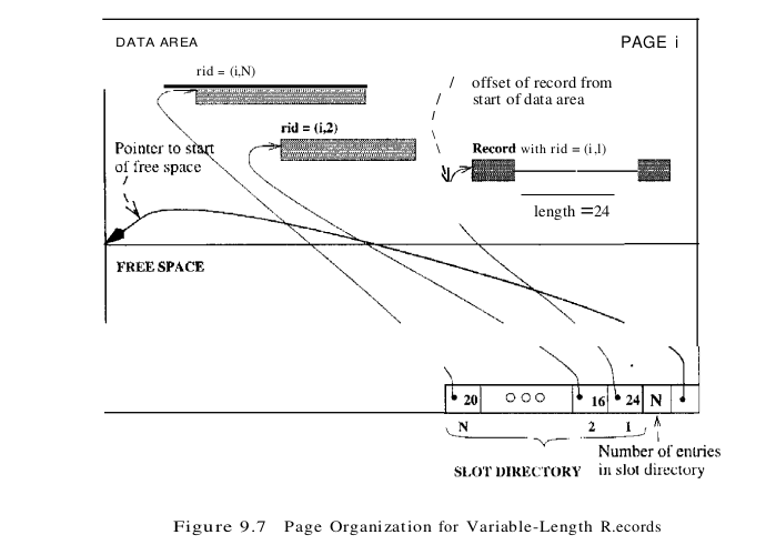
If records are of variable length, then we cannot divide the page into a fixed collection of slots. The problem is that, when a new record is to be inserted, we have to find an empty slot of just the right length – if we use a slot that is too big, we waste space, and obviously we cannot use a slot that is smaller than the record length. Therefore, when a record is inserted, we must allocate just the right amount of space for it, and when a record is deleted, we must move records to fill the hole created by the deletion, to ensure that all the free space on the page is contiguous. Therefore, the ability to move records on a page becomes very important. The most flexible organization for variable-length records is to maintain a directory of slots for each page, with a (record offset, record length) pair per slot. The first component (record offset) is a ‘pointer’ to the record, as shown in Figure 9.7; it is the offset in bytes from the start of the data area on the page to the start of the record, Deletion is readily accomplished by setting the record offset to -1. Records can be moved around on the page because the rid, which is the page number and slot number (that is, position in the directory), does not change when the record is moved; only the record offset stored in the slot changes.

The space available for new records must be managed carefully because the page is not preformatted into slots. One way to manage free space is to maintain a pointer (that is, offset from the start of the data area on the page) that indicates the start of the free space area. When a new record is too large to fit into the remaining free space, we have to move records on the page to reclaim the space freed by records deleted earlier. The idea is to ensure that, after reorganization, all records appear in contiguous order, followed by the available free space.

Record Formats

While choosing a way to organize the fields of a record, we must take into account whether the fields of the record are of fixed or variable length and consider the cost of various operations on the record, including retrieval and modification of fields.

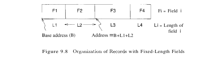
In a fixed-length record, each field has a fixed length (that is, the value in this field is of the same length in all records), and the number of fields is also fixed. The fields of such a record can be stored consecutively, and, given the address of the record, the address of a particular field can be calculated using information about the lengths of preceding fields, which is available in the system catalog. This record organization is illustrated in Figure 9.8.

In the relational model, every record in a relation contains the same number of fields. If the number of fields is fixed, a record is of variable length only because some of its fields are of variable length. One possible organization is to store fields consecutively, separated by delimiters (which are special characters that do not appear in the data itself). This organization requires a scan of the record to locate a desired field. An alternative is to reserve some space at the beginning of a record for use as an array of integer offsets – the ith integer in this array is the starting address of the ith field value relative to the start of the record. Note that we also store an offset to the end of the record; this offset is needed to recognize where the last held ends. Both alternatives are illustrated in Figure 9.9.

The second approach is typically superior. For the overhead of the offset array, we get direct access to any field. We also get a clean way to deal with null values. A null value is a special value used to denote that the value for a field is unavailable or inapplicable. If a field contains a null value, the pointer to the end of the field is set to be the same as the pointer to the beginning of the field. That is, no space is used for representing the null value, and a comparison of the pointers to the beginning and the end of the field is used to determine that the value in the field is null. Variable-length record formats can obviously be used to store fixed-length records as well; sometimes, the extra overhead is justified by the added flexibility, because issues such as supporting null values and adding fields to a record type arise with fixed-length records as well. Having variable-length fields in a record can raise some subtle issues, especially when a record is modified.

• Modifying a field may cause it to grow, which requires us to shift all subsequent fields to make space for the modification in all three record formats just presented.
• A modified record may no longer fit into the space remaining on its page. If so, it may have to be moved to another page. If rids, which are used to ‘point’ to a record, include the page number, moving a record to another page causes a problem. We may have to leave a ‘forwarding address’ on this page identifying the new location of the record. And to ensure that space is always available for this forwarding address, we would have to allocate some minimum space for each record, regardless of its length.
• A record may grow so large that it no longer fits on anyone page. We have to deal with this condition by breaking a record into smaller records. The smaller records could be chained together-part of each smaller record is a pointer to the next record in the chain—to enable retrieval of the entire original record.