- Introduction to Schema Refinement
- Decompositions
- Function dependencies
- Reasoning About FD
- Normal Forms
- Properties of Decompositions
- Normalization
- Schema Refinement in Database Design
- Other Kinds of Dependencies
Conceptual database design gives us a set of relation schemas and integrity constraints (ICs) that can be regarded as a good starting point for the final database design. This initial design must be refined by taking the ICs into account more fully than is possibly with just the ER model constructs and also by considering performance criteria and typical workloads.
We concentrate on an important class of constraints called functional dependencies. Other kinds of ICs, for example, multivalued dependencies and join dependencies, also provide useful information. They can sometimes reveal redundancies that cannot be detected using functional dependencies alone. We discuss these other constraints briefly.
Introduction to Schema Refinement
We now present an overview of the problems that schema refinement is intended to address and a refinement approach based on decompositions. Redundant storage of information is the root cause of these problems. Although decomposition can eliminate redundancy, it can lead to problems of its own and should be used with caution.
Problems Caused by Redundancy
Storing the same information redundantly, that is, in more than one place within a database, can lead to several problems:
- Redundant Storage: same information is stored repeatedly.
- Update Anomalies: If one copy of such repeated data is updated, an inconsistency is created unless all copies are similarly updated.
- Insertion Anomalies: It may not be possible to store certain information unless some other, unrelated, information is stored as well.
- Deletion Anomalies: It may not be possible to delete certain information without losing some other, unrelated, information as well.
Consider a relation obtained by translating a variant of the Hourly_Emps entity set
Hourly_Emps(ssn, name, lot, rating, hourly_wages, hours_worked)
The key for Hourly_Emps is ssn. In addition, suppose that the hourly_wages attribute is determined by the rating attribute. That is, for a given rating value, there is only one permissible hourly_wages value. This IC is an example of a functional dependency. It leads to possible redundancy in the relation Hourly_Emps, as illustrated in Figure 19.1.
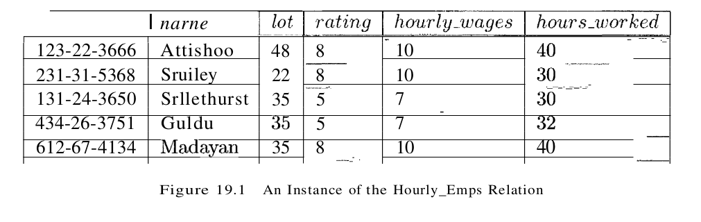
If the same value appears in the rating column of two tuples, the IC tells us that the same value must appear in the hourly_wages column as well. This redundancy has the same negative consequences as before:
- Redundant Storage: the rating value 8 corresponds to the hourly wage 10, and this association is repeated three times.
- Update Anoma1ies: The hourly_wages in the first tuple could be updated without making a similar change in the second tuple.
- Insertion Anomalies: We cannot insert a tuple for an employee unless we know the hourly_wage for the employee’s rating value.
- Deletion Anomalies: If we delete all tuples with a given rating value (e.g., we delete the tuples for Smethurst and Guldu) we lose the association between that rating value and its hourly_wage value.
Ideally, we want schemas that do not permit redundancy, but at the very least we want to be able to identify schemas that do allow redundancy. Even if we choose to accept a schema with some of these drawbacks, perhaps owing to performance considerations, we want to make an informed decision.
It is worth considering whether the use of null values can address some of these problems. As we will see in the context of our example, they cannot provide a complete solution, but they can provide some help.
Consider the example Hourly_Emps relation. Clearly, null values cannot help eliminate redundant storage or update anomalies. It appears that they can address insertion and deletion anomalies. For instance, to deal with the insertion anomaly example, we can insert an employee tuple with null values in the hourly wage field. However, null values cannot address all insertion anomalies. For example, we cannot record the hourly wage for a rating unless there is an employee with that rating, because we cannot store a null value in the ssn field, which is a primary key field. Similarly, to deal with the deletion anomaly example, we might consider storing a tuple with null values in all fields except rating and hourly_wages if the last tuple with a given rating would otherwise be deleted. However, this solution does not work because it requires the ssn, value to be null, and primary key fields cannot be null. Thus, null values do not provide a general solution to the problems of redundancy, even though they can help in some cases.
Decompositions
Intuitively, redundancy arises when a relational schema forces an association between attributes that is not natural. Functional dependencies (and, for that matter, other ICs) can’t be used to identify such situations and suggest refinements to the schema. The essential idea is that many problems arising from redundancy can be addressed by replacing a relation with a collection of smaller relations.
A decomposition of a relation schema R consists of replacing the relation schema by two (or one) relation schemas that each contain a subset of the attributes of R and together include all attributes in R. Intuitively, we want to store the information in any given instance of R by storing projections of the instance. This section examines the use of decompositions through several examples. We can decompose Hourly_Emps into two relations:
Hourly_Emps2(ssn, name, lot, rating, hours_worked)
Wages(rating, hourly_wages)
The instances of these relations corresponding to the instance of Hourly_Emps relation in Figure 19.1 is shown in Figure 19.2.

Note that we can easily record the hourly wage for any rating simply by adding a tuple to Wages, even if no employee with that rating appears in the current instance of Hourly_Emps. Changing the wage associated with a rating involves updating a single Wages tuple. This is more efficient than updating several tuples (as in the original design), and it eliminates the potential for inconsistency.
Problems related to Decomposition
Unless we are careful, decomposing a relation schema can create more problems than it solves. Two important questions must be asked repeatedly:
- Do we need to decompose a relation?
- What problems (if any) does a given decomposition cause?
To help with the first question, several normal forms have been proposed for relations. If a relation schema is in one of these normal forms, we know that certain kinds of problems cannot arise. Considering the normal form of a given relation schema can help us to decide whether or not to decompose it further. If we decide that a relation schema msut be decomposed further, we must choose a particular decomposition (I.e., a particular collection of smaller relations to replace the given relation).
With respect to the second question, two properties of decompositions are of particular interest. The lossless-join property enables us to recover any instance of the decomposed relation from corresponding instances of the smaller relations. The dependency-preservation property enables us to enforce any constraint on the original relation by simply enforcing same contraints on each of the smaller relations. That is, we need not perform joins of the smaller relations to check whether a constraint on the original relation is violated. From a performance standpoint, queries over the original relation may require us to join the decomposed relations. If such queries are common, the performance penalty of decomposing the relation may not be acceptable. In this case, we may choose to live with some of the problems of redundancy and not decompose the relation. It is important to be aware of the potential problems caused by such residual redundancy in the design and to take steps to avoid them (e.g., by adding same checks to application code). In some situations, decomposition could actually improve performance. This happens, for example, if most queries and updates examine only one of the decomposed relations, which is smaller than the original relation. Our goal in this chapter is to explain some powerful concepts and design guidelines based on the theory of functional dependencies.
A good database designer should have a firm grasp of normal forms and what problems they (do or do not) alleviate, the technique of decomposition, and potential problems with decompositions. For example, a designer often asks questions such as these: Is a relation in a given normal form? Is a decomposition dependency-preserving? Our objective is to explain when to raise these questions and the significance of the answers.
Function dependencies
A functional dependency (FD) is a kind of IC that generalizes the concept of a key. Let R be a relation schema and let X and Y be nonempty sets of attributes in R. We say that an instance r of R satisfies the FD $X \rightarrow Y$ if the following holds for every pair of tuples t1 and t2 in r.
If t1.X = t2.X, then t1.Y = t2.Y
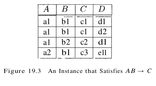
We use the notation t1.X to refer to the projection of tuple t1 onto the attributes in X, in a natural extension of our TRC notation t.a for referring to attribute a of tuple t. An FD $X \rightarrow Y$ essentially says that if two tuples agree on the values in attributes X, they must also agree on the values in attributes Y. Figure 19.3 illustrates the meaning of the FD $AB \rightarrow C$ by showing an instance that satisfies this dependency. The first two tuples show that an FD is not the same as a key constraint: Although the FD is not violated, AB is clearly not a key for the relation. The third and fourth tuples illustrate that if two tuples differ in either the A field or the B field, they can differ in the C field without violating the FD. On the other hand, if we add a tuple (a1, b1, c2, d1) to the instance shown in this figure, the resulting instance would violate the FD; to see this violation, compare the first tuple in the figure with the new tuple.
Recall that a legal instance of a relation must satisfy all specified ICs, including all specified FDs. By looking at an instance of a relation, we might be able to tell that a certain FD does not hold. However, we can’t never deduce that an FD does hold by looking at one or more instances of the relation, because an FD, like other ICs, is a statement about all possible legal instances of the relation. A primary key constraint is a special case of an FD. The attributes in the key play the role of X, and the set of all attributes in the relation plays the role of Y. Note, however, that the definition of an FD does not require that the set X be minimal; the additional minimality condition must be met for X to be a key. If $X \rightarrow Y$ holds, where Y is the set of all attributes, and there is some (strictly contained) subset V of X such that $V \rightarrow Y$ holds, then X is a supeerkey.
Reasoning About FD
Given a set of FDs over a relation schema R, typically several additional FDs hold over R whenever all of the given FDs hold. As an example, consider:
Workers(ssn, name, lot, did, since)
We know that ssn $\rightarrow$ did holds, since ssn is the key, and FD did $\rightarrow$ lot is given to hold. Therefore, in any legal instance of Workers, if two tuples have the same ssn value, they must have the same did value (from the first FD), and because they have the same did value, they must also have the same lot value (from the second FD). Therefore, the FD ssn $\rightarrow$ lot also holds on Workers. We say that an FD f is implied by a given set F of FDs if f holds on every relation instance that satisfies all dependencies in F; that is, f holds whenever all FDs in F hold. Note that it is not sufficient for f to hold on some instance that satisfies all dependencies in F; rather, f must hold on every instance that satisfies all dependencies in F.
Closure of a Set of FDs
The set of all FDs implied by a given set F of FDs is called the closure of F, denoted as $F^+$. An important question is how we can infer, or compute, the closure of a given set F of FDs. The answer is simple and elegant. The following three rules, called Armstrong’s Axioms, can be applied repeatedly to infer all FDs implied by a set F of FDs. We use X, Y, and Z to denote sets of attributes over a relation schema R:
- Reflexivity: if $X \supseteq Y$, then $X \rightarrow Y$
- Augmentation: if $X \rightarrow Y$, then $XZ \rightarrow YZ$ for any Z
- Transitivity: if $X \rightarrow Y$ and $Y \rightarrow Z$, then $X \rightarrow Z$
Theorem 1 Armstrong’s Axioms are sound, in that they generate only FDs in $F^{+}$ when applied to a set $\mathrm{F}$ of FDs. They are also complete, in that repeated application phase rules will generate all $F D s$ in the closure $F^+$.
It is convenient to use some additional rules while reasoning about $F^+$:
- Union: if $X \rightarrow Y$ and $X \rightarrow Z$, then $X \rightarrow YZ$
- Decomposition: if $X \rightarrow YZ$, then $X \rightarrow Y$ and $X \rightarrow Z$
To illustrate the use of these inference rules for FDs, consider a relation schema ABC with FDs A $\rightarrow$ B and B $\rightarrow$ C. In a trivial FD, the right side contains only attributes that also appear on the left side; such dependencies always hold due to reflexivity. Using reflexivity, we can generate all trivial dependencies, which are of the form:
\[X \rightarrow \mathrm{Y} \text {, where } \mathrm{Y} \subseteq X, X \subseteq A B C \text {, and } \mathrm{Y} \subseteq A B C \text {. }\]From transitivity we get A $\rightarrow$ C. From augmentationw we get the nontrivial dependencies:
\[A C \rightarrow B C, A B \rightarrow A C, A B \rightarrow C B\]As another example, we use a more elaborate version of Contracts:
Contracts(constractid, supplierid, projectid, deptid, partid, qty, value)
We denote the schema for Contracts as CSJDPQV. The meaning of a tuple is that the contract with contractid C is an agreement that supplier S (supplierid) will supply Q items of part P (partid) to project J (pojectid) associated with department D (deptid); the value V of this contract is equal to value.
The following ICs are known to hold:
- The contract id C is a key: C $\rightarrow$ CSJDPQV.
- A project purchases a given part using a single contract: D $\rightarrow$ C
- A department purchases at most one part from a supplier: SD $\rightarrow$ P
Several additional FDs hold in the closure of the set of given FDs:
From $ D \rightarrow C, C \rightarrow C S J D P Q V$, and transitivity, we infer $ D \rightarrow C S J D P Q V$. From SD $\rightarrow P$ and augmentation, we infer $S D J \rightarrow J P$.
Attribute Closure
If we just want to check whether a given dependency, say, X $\rightarrow$ Y, is in the closure of a set F of FDs, we can do so efficiently without computing $F^+$. We first compute the attribute closure $X^+$ with respect to F, which is the set of attributes A such that X $\rightarrow$ A can be inferred using the Armstrong Axioms. The algorithm for computing the attribute closure of a set X of attributes is shown in Figure 19.4.
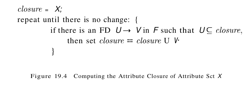
Theorem 2 The algorithm shown in figure 19.4 computes the attribute closure $X^+$ of the attribute set X with respect to the sct of FDs F.
Normal Forms
Given a relation schema, we need to decide whether it is a good design or we need to decompose it into smaller relations. Such a decision must be guided by an understanding of what problems, if any, arise from the current schema. To provide such guidance, several normal forms have been proposed. If a relation schema is in one of these normal forms, we know that certain kinds of problems cannot arise. The normal forms based on FDs are first normal form (1NF), second normal form (2NF), third normal form (3NF) , and Boyce-Codd normal form (BCNF). These forms have increasingly restrictive requirements: Every relation in BCNF is also in 3NF, every relation in 3NF is also in 2NF, and every relation in 2NF is in 1NF.
A relation is in first normal form if every field contains only atomic values, that is, no lists or sets. This requirement is implicit in our definition of the relational mode. Although some of the newer database systems are relaxing this requirement, in this chapter we assume that it always holds. 2NF is mainly of historical interest. 3NF and BCNF are important from a database design standpoint. While studying normal forms, it is important to appreciate the role played by FDs. Consider a relation schema R with attributes ABC. In the absence of any ICs, any set of ternary tuples is a legal instance and there is no potential for redundancy. On the other hand, suppose that we have the FD A $\rightarrow$ B. Now if several tuples have the same A value, they must also have the same B value. This potential redundancy can be predicted using the FD information. If more detailed ICs are specified, we may be able to detect more subtle redundancies as well. We primarily discuss redundancy revealed by FD information.
Boyce-Codd Normal Form
Let R be a relation schema, F be the set of FDs given to hold over R, X be a subset of the attributes of R, and A be an attribute of R. R is in Boyce-Codd normal form if, for every FD X $\rightarrow$ A in F, one of the following statements is true:
- $A \in X$; that is, it is a trivial $\mathrm{FD}$
- or $X$ is a superkey.
Intuitively, in a BCNF relation, the only nontrivial dependencies are those in which a key determines some attribute(s). Therefore, each tuple can be thought of as an entity or relationship, identified by a key and described by the remaining attributes. Each attribute must describe an entity or relationship identified by the key, the whole key, and nothing but the key. If we use ovals to denote attributes or sets of attributes and draw arcs to indicate FDs, a relation in BCNF has the structure illustrated in Figure 19.5, considering just one key for simplicity. (If there are several candidate keys, each candidate key can play the role of KEY in the figure, with the other attributes being the ones not in the chosen candidate key.)

BCNF ensures that no redundancy can be detected using FD information alone. It is thus the most desirable normal form (from the point of view of redundancy) if we take into account only FD information. This point is illustrated in Figure 19.6.
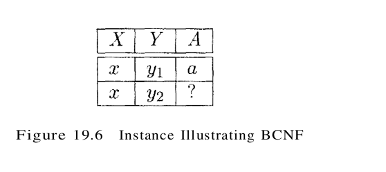
This figure shows (two tuples in) an instance of a relation with three attributes X, Y, and A. There are two tuples with the same value in the X column. Now suppose that we know that this instance satisfies an FD X $\rightarrow$ A. We can see that one of the tuples has the value a in the A column. What can we infer about the value in the A column in the second tuple? Using the FD, we can conclude that the second tuple also has the value a in this column. (Note that this is really the only kind of inference we can make about values in the fields of tuples by using FDs.) But is this situation not an example of redundancy? We appear to have stored the value a twice. Can such a situation arise in a BCNF relation? The answer is No! If this relation is in BCNF, because A is distinct from X, it follows that X must be a key. (Otherwise, the FD X $\rightarrow$ A would violate BCNF.) If X is a key, then Y1 = Y2, which means that the two tuples are identical since a relation is defined to be a set of tuples, we cannot have two copies of the same tuple and the situation shown in Figure 19.6 cannot arise. Therefore, if a relation is in BCNF, every field of every tuple records a piece of information that cannot be inferred (using only FDs) from the values in all other fields in (all tuples of) the relation instance.
Third Normal Form
Let R be a relation schema, F be the set of FDs given to hold over R, X be a subset of the attributes of R, and A be an attribute of R. R is in third normal form if, for every FD X $\rightarrow$ A in F, one of the following statements is true:
- $A \in X, that is it is a trivial FD$
- of X is a superkey
- or A is part of some key for R.
The definition of 3NF is similar to that of BCNF, with the only difference being the third condition. Every BCNF relation is also in 3NF. To understand the third condition, recall that a key for a relation is a minimal set of attributes that uniquely determines all other attributes. A must be part of a key (any key, if there are several). It is not enough for A to be part of a superkey, because the latter condition is satisfied by every attribute. Finding all keys of a relation schema is known to be an NP-complete problem, and so is the problem of determining whether a relation sehema is in 3NF. Suppose that a dependency X $\rightarrow$ A causes a violation of 3NF. There are two cases:
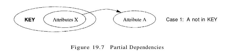
- X is a proper subset of some key K. Such a dependency is sometimes called a partial dependency. In this case, we store (X, A) pairs redundantly. As an example, consider the Reserves relation with attributes SBDC. The only key is SBD, and we have the FD S $\rightarrow$ C. We store the credit card number for a sailor as many times as there are reservations for that sailor.
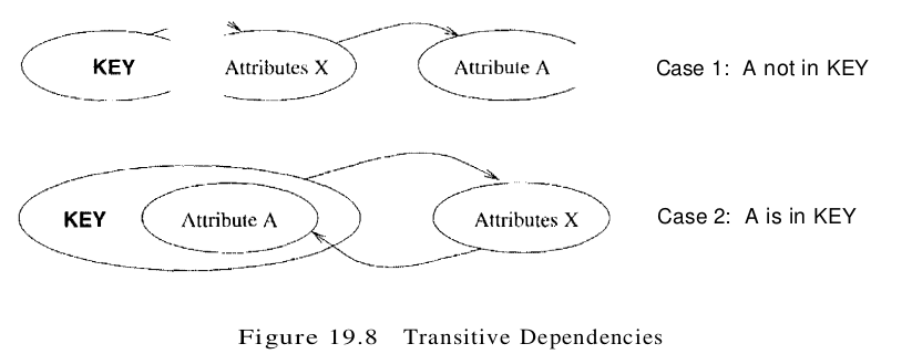
- X is not a prober subset of any key. Such a dependency is sometimes called a transitive dependency, because it means we have a chain of dependencies X $\rightarrow$ A. The problem is that we cannot associate an X value with a K value unless we also associate an A value with an X value. As an example, consider the Hourly_Emps relation with attributes SNLRWH. The only key is S, but there is an FD R $\rightarrow$ W, which gives rise to the chain S $\rightarrow$ R $\rightarrow$ W. The consequence is that we cannot record the fact that employee S has rating R without knowing the hourly wage for that rating. This condition leads to insertion, deletion, and update anomalies.
Partial dependencies are illustrated in Figure 19.7, and transitive dependencies are illustrated in Figure 19.8. Note that in Figure 19.8, the set X of attributes may or may not have some attributes in common with KEY; the diagram should be interpreted as indicating only that X is not a subset of KEY.
The motivation for 3NF is rather technical. By making an exception for certain dependencies involving key attributes, we can ensure that every relation schema can be decomposed into a collection of 3NF relations using only decompositions that have certain desirable properties. Such a guarantee does not exist for BCNF relations; the 3NF definition weakens the BCNF requirements just enough to make this guarantee possible. We may therefore compromise by settling for a 3NF design. We may sometimes accept this compromise (or even settle for a non-3NF schema) for other reasons as well. Unlike BCNF, however, some redundancy is possible with 3NF. The problems associatted with partial and transitive dependencies persist if there is a nontrivial dependency X $\rightarrow$ A and X is not a superkey, even if the relation is in 3NF bccause A is part of a key.
To understand this point, let us revisit the Reserves relation with attributes SBDC and the FD S $\rightarrow$ C, which states that a sailor uses a unique credit card to pay for reservations. S is not a key, and C is not part of a key. (In fact, the only key is SBD.) Hence, this relation is not in 3NF; (S, C) pairs are stored redundantly. However, if we also know that credit cards uniquely identify the owner, we have the FD C $\rightarrow$ S, which means that CBD is also a key for Reserves. Therefore, the dependency S $\rightarrow$ C does not violate 3NF, and Reserves is in 3NF. Nonetheless, in all tuples containing the same S value, the same (S, C) pair is redundantly recorded.
For completeness, we remark that the definition of second normal form is essentially that partial dependencies are not allowed. Thus, if a relation is in 3NF (which precludes both partial and transitive dependencies), it is also in 2NF.
Properties of Decompositions
Lossless-Join Decomposition
Let R be a relation schema and let F be a set of FDs over R. A decomposition of R into two schemas with attribute sets X and Y is said to be a lossless-join decomposition with respect to F if, for every instance T of R that satisfies the dependencies in F, $\pi_{X}(r) \bowtie \pi_{Y}(r)=T$. In other words, we can recover the original relation from the decomposed relations.
This definition can easily be extended to cover a decomposition of R into more than two relations. It is easy to see that $T \subseteq \pi_{X}(r) \bowtie \pi_{Y}(r)$ always holds. In general, though, the other direction does not hold. If we take projections of a relation and recombine them using natural join, we typically obtain some tuples that were not in the original relation. This situation is illustrated in Figure 19.9.

By replacing the instance T shown in Figure 19.9 with the instances $\pi_{SP}(r)$ and $\pi_{PD}(r)$, we lose some information. In particular, suppose that the tuples in r denote relationships. We can no longer tell that the relationships (S1, P1, D3 ) and (S3, P1, D1) do not hold. The decomposition of schema SPD into SP and PD is therefore loss, if the instance r shown in the figure is legal, that is, if this instance could arise in the enterprise being modeled. All decompositions used to eliminate redundancy must be lossless. The following simple test is very useful:
Theorem 3 Let R be a relation and F be a set of FDs that hold over R. The decomposition of R into relations with attribute sets R1 and R2 is loseless if and only if $F^+$ contains either the FD R1 $\cap$ R2 $\rightarrow$ R1 or the FD R1 $\cap$ R2 $\rightarrow$ R2.
In other words, the attributes common to R1 and R2 must contain a key for either R1 or R2. If a relation is decomposed into more than two relations, an efficient (time polynomial in the size of the dependency set) algorithm is available to test whether or not the decomposition is lossless, but we will not discuss it.
Consider the Hourly_Emps relation again(Hourly_Emps(ssn, name, lot, rating, hourly_wages, hours_worked)). It has attributes SNLRWH, and the FD R $\rightarrow$ W causes a violation of 3NF. We dealt with this violation by decomposing the relation into SNLRH and RW. Since R is common to both decomposed relations and R $\rightarrow$ W holds, this decomposition is lossless-join.
This example illustrates a general observation that follows from Theorem 3: If an FD X $\rightarrow$ Y holds over a relation R and X $\cap$ Y is empty, the decomposition of R into R - Y and XY is lossless. X appears in both R - Y(since X $\cap$ Y is empty) and XY, and then X is a key for XY.
Another important observation, which we state without proof, has to do with repeated decomposition. Suppose that a relation R is decornposed into R1 and R2 through a lossless-join decomposition, and that R1 is decomposed into R11 and R12 through another lossless-join decomposition. Then, the decomposition of R into R11, R12, and R2 is lossless-join; by joining R11 and R12, we can recover R1, and by then joining R1 and R2, we can recover R.
Dependency-Preserving Decomposition
Consider the Contracts relation(Contracts(constractid, supplierid, projectid, deptid, partid, qty, value)) with attributes CSJDPQV. The given FDs are C $\rightarrow$ CSJDPQV, JP $\rightarrow$ C and SD $\rightarrow$ P. Because SD is not a key the dependency SD $\rightarrow$ P causes a violation of BCNF.
We can decompose Contracts into two relations with schelnas CSJDQV and SDP to address this violation; the decomposition is lossless-join. There is one subtle problem, however. We can enforce the integrity constraint JP $\rightarrow$ C easily when a tuple is inserted into Contracts by ensuring that no existing tuple has the same JP values (as the inserted tuple) but different C values. Once we decompose Contracts into CSJDQV and SDP, enforcing this constraint requires an expensive join of the two relations whenever a tuple is inserted into CSJDQV. We say that this decomposition is not dependency-preserving. Intuitively, a dependency-preserving decomposition allows us to enforce all FDs by examining a single relation instance on each insertion or modification of a tuple. (Note that deletions cannot cause violation of FDs.) To define dependency-preserving decompositions precisely, we have to introduce the concept of a projection of FDs. Let R be a relation schema that is decomposed into two schemas with attribute sets X and Y, and let F be a set of FDs over R. The projection of F on X is the set of FDs in the closure $F^+$ (not just F !) that involve only attributes in X. We denote the projection of F on attributes of X as $F_x$. Note that a dependency U $\rightarrow$ V in $F^+$ is in $F_x$; only if all the attributes in U and V are in X.
The decomposition of relation schema R with FDs F into schemas with attribute sets X and Y is dependency-preserving if $\left(F_{X} \cup F_{Y}\right)^{+}=F^{+}$. That is, if we take the dependencies in $F_{X}$ and $F_{Y}$ and compute the closure of their union, we get back all dependencies in the closure of F. Therefore, we need to enforce only the dependencies in $F_{X}$ and $F_{Y}$; all FDs in $F^+$ are then sure to be satisfied. To enforce $F_x$, we need to examine only relation X (on inserts to that relation). To enforce $F_y$, we need to examine only relation Y.
To appreciate the need to consider the closure $F^+$ while computing the projection of f, suppose that a relation R with attributes ABC is decomposed into relations with attributes AB and BC. The set F of FDs over R includes A $\rightarrow$ B, B $\rightarrow$ C, and C $\rightarrow$ A. Of these, A $\rightarrow$ B is in $F_{AB}$ and B $\rightarrow$ C is in $F_{BC}$. But is this decomposition dependency-preserving? What about C $\rightarrow$ A? This dependency is not implied by the dependencies listed (thus far) for $F_{AB}$ and $F_{BC}$. The closure of F contains all dependencies in F plus A $\rightarrow$ C, B $\rightarrow$ A, and C $\rightarrow$ B. Consequently, $F_{AB}$ also contains B $\rightarrow$ A, and $F_{BC}$ contains C $\rightarrow$ B. Therefore, $F_{AB} \cup F_{BC}$ contains A $\rightarrow$ B, B $\rightarrow$ C, B $\rightarrow$ A, and C $\rightarrow$ B. The closure of the dependencies in $F_{AB}$ and $F_{BC}$ now includes C $\rightarrow$ A (which follows from C $\rightarrow$ B, B $\rightarrow$ A, and transitivity). Thus, the decomposition preserves the dependency C $\rightarrow$ A.
Normalization
Decomposition into BCNF
We now present an algorithm for decomposing a relation schema R with a set of FDs F into a collection of BCNF relation schemas:
- Suppose that R is not in BCNF. Let X $\subseteq$ R, A be a single attribute in R, and X $\rightarrow$ A be an FD that causes a violation of BCNF. Decompose R into R - A and XA.
- If either R - A or XA is not in BCNF, decompose them further by a recursive application of this algorithm.
R - A denotes the set of attributes other than A in R, and XA denotes the union of attributes in X and A. Since X $\rightarrow$ A violates BCNF, it is not a trivial dependency; further, A is a single attribute. Therefore, A is not in X; that is X $\cap$ A is empty. Therefore, each decomposition carried out in Step 1. is lossless-join. The set of dependencies associated with R - A and XA is the projection of F onto their attributes. If one of the new relations is not in BCNF, we decompose it further in Step 2. Since a decomposition results in relations with strictly fewer attributes, this process terminates, leaving us with a collection of relation schemas that are all in BCNF. Further, joining instances of the (two or more) relations obtained through this algorithm yields precisely the corresponding instance of the original relation (i.e., the decomposition into a collection of relations each of which in BCNF is a lossless-join decomposition). Consider the Contracts relation(Contracts(constractid, supplierid, projectid, deptid, partid, qty, value)) with attributes CAJDPQV and key C. We are given FDs JP $\rightarrow$ C and SD $\rightarrow$ P. By using the dependency SD $\rightarrow$ P to guide the decomposition, we get the two schemas SDP and CSJDQV. SDP is in BCNF. Suppose that we also have the constraint that each project deals with a single supplier: J $\rightarrow$ S. This means that the schema CSJDQV is not in BCNF. So we decompose it further into JS and CJDCQV. C $\rightarrow$ JDQV holds over CJDQV; the only other FDs that hold are those obtained from this FD by augmentation, and therefore all FDs contain a key in the left side. Thus, each of the schemas SDP, JS, and CJDQV is in BCNF and this collection of schemas also represents a lossless-join decomposition of CSJDQV.
The steps in this decomposition process can be visualized as a tree, as shown in Figure 19.10. The root is the original relation CSJDPQV, and the leaves are the BCNF relations that result from the decomposition algorithm: SDP, JS, and CJDQV. Intuitively, each internal node is replaced by its children through a single decomposition step guided by the FD shown just below the node.

The decomposition of CSJDQPV into SDP, JS, and CJDQV is not dependency-preserving. Intuitively, dependency JP $\rightarrow$ C can’t be enforced without a join. One way to deal with this situation is to add a relation with attributes CJP. In effect, this solution amounts to storing some information redundantly to make the dependency enforcement cheaper.
This is a subtle point: Each of the schemas CJP, SDP, JS, and CJDQV is in BCNF, yet some redundancy can be predicted by FD information. In particular, if we join the relation instances for SDP and CJDQV and project the result onto the attributes CJP, we must get exactly the instance stored in the relation with schema CJP. This example shows that redundancy can still occur across relations, even though there is no redundancy within a relation.
Decomposing to 3NF
Clearly, the approach we outlined for lossless-join decomposition into BCNF also gives us a lossless-join decomposition into 3NF. (Typically, we can stop a little earlier if we are satisfied with a collection of 3NF relations.) But this approach does not ensure dependency-preservation.
A simple modification, however, yields a decomposition into 3NF relations that is lossless-join and dependency-preserving. Before we describe this modification, we need to introduce the concept of a minimal cover for a set of FDs.
A minimal cover for a set F of FDs is a set G of FDs such that:
- Every dependency in G is of the form X $\rightarrow$ A, where A is a single attribute.
- The closure $F^+$ is equal to the closure $G^+$.
- If we obtain a set U of dependencies from G by deleting one or more dependencies or by deleting attributes from a dependency in G, then $F^+ \neq U^+$.
Intuitively, a minimal cover for a set F of FDs is an equivalent set of dependencies that is minimal in two respects: (1) Every dependency is as small as possible; that is each attribute on the left side is necessary and the right side is a single attribute. (2) Every dependency in it is required for the closure to be equal to $F^+$.
As an example, let F be the set of dependencies:
A $\rightarrow$ B, ABCD $\rightarrow$ E, EF $\rightarrow$ G, EF $\rightarrow$ H and ACDF $\rightarrow$ BG
First let us rewrite it ACDF $\rightarrow$ BG so that every right side is a single attribute:
ACDF $\rightarrow$ B and ACDF $\rightarrow$ G
Next consider ACDF $\rightarrow$ G, This dependency is implied by the following FDs:
A $\rightarrow$ B, ABCD $\rightarrow$ E, and EF $\rightarrow$ G
Therefore, we can delete it. Similarly, we can delete ACDF $\rightarrow$ B. Next consider ABCD $\rightarrow$ E. Since A $\rightarrow$ B holds, we can replace it with ACD $\rightarrow$ E, (At this point, the reader should verify that each remaining FD is minimal and required,) Thus, a minimal cover for F is the set:
A $\rightarrow$ B, ACD $\rightarrow$ E, EF $\rightarrow$ G, and EF $\rightarrow$ H
The preceding example illustrates a general algorithm for obtaining a minimal cover of a set F of FDs:
- Put the FDs in a Standard Form: Obtain a collection G of equivalent FDs with a single attribute on the right side (using the decomposition axiom),
- Minimize the Left Side of Each FD: For each FD in G, check each attribute in the left side to see if it can be deleted while preserving equivalence to F+,
- Delete Redundant FDs: Check each remaining FD in G to see if it can be deleted while preserving equivalence to $F^+$.
Note that the order in which we consider FDs while applying these steps could produce different minimal covers; there could be several minimal covers for a given set of FDs. More important, it is necessary to minimize the left sides of FDs before checking for redundant FDs. If these two steps are reversed, the final set of FDs could still contain some redundant FDs (i,e., not be a minimal cover), as the following example illustrates. Let F be the set of dependencies, each of which is already in the standard form:
ABCD $\rightarrow$ E, E $\rightarrow$ D, A $\rightarrow$ B and AC $\rightarrow$ D
Observe that none of these FDs is redundant; if we checked for redundant FDs first, we would get the same set of FDs F. The left side of ABCD $\rightarrow$ E can be replaced by AC while preserving equivalence to $F^+$, and we would stop here if we checked for redundant FDs in F before minimizing the left sides. However, the set of FDs we have is not a minimal cover:
AC $\rightarrow$ E, E $\rightarrow$ D, A $\rightarrow$ B and AC $\rightarrow$ D
From transivity, the first two FDs imply the last FD, which can therefore be deleted while preserving equivalence to $F^+$. The important point to note is that AC $\rightarrow$ D becomes redundant only after we replace ABCD $\rightarrow$ E with AC $\rightarrow$ E. If we minimize left sides of FDs first and then cheek for redundant FDs, we are left with the first three FDs in the preeeding list, which is indeed a minimal cover for F.
Dependency-Preserving Decomposition into 3NF
Returning to the problem of obtaining a lossless-join, dependency-preserving decomposition into 3NF relations, let R be a relation with a set F of FDs that is a minimal cover, and let $R_1$, $R_2$, … , $R_n$ be a lossless-join decomposition of R. For 1 < i < n, suppose that each $R_i$ is in 3NF and let $F_i$ denote the projection of F onto the attributes of $R_i$. Do the following:
- Identify the set N of dependencies in F that is not preserved, that is, not included in the closure of the union of $F_i$s.
- For each FD X $\rightarrow$ A in N, create a relation schema XA and add it to the decomposition of R.
Obviously, every dependency in F is preserved if we replace R by the $R_i$s plus the schemas of the form XA added in this step. The $R_i$s are given to be in 3NF. We can show that each of the schemas XA is in 3NF as follows: Since X $\rightarrow$ A is in the minimal cover F, Y $\rightarrow$ A does not hold for any Y that is a strict subset of X. Therefore, X is a key for XA. Further, if any other dependencies hold over XA, the right side can involve only attributes in X because A is a single attribute (because X $\rightarrow$ A is an FD in a minimal cover). Since X is a key for XA, none of these additional dependencies causes a violation of 3NF (although they might cause a violation of BCNF).
As an optimization, if the set N contains several FDs with the same left side, say, X $\rightarrow A_1 $, X $\rightarrow A_2$, …, X $\rightarrow A_n$, we can replace them with a single equivalent FD X $\rightarrow A_1…A_n$. Therefore, we produce one relation schema X$A_1…A_n$, instead of several schemas $XA_1$, …. $XA_n$, which is generally preferable.
Consider the Contracts relation with attributes CSJDPQV and FDs JP $\rightarrow$ C, SD $\rightarrow$ P and J $\rightarrow$ S. If we decompose CSJDPQV into SDP and CSJDQV, then SDP is in BCNF, but CSJDQV is not even in 3NF. So we decompose it further into JS and CJDQV. The relation schemas SDP, JS, and CJDQV are in 3NF (in fact, in BCNF) and the decomposition is lossless-join. However, the dependency JP $\rightarrow$ C is not preserved. This problem can be addressed by adding a relation schema CJP to the decomposition.
3NF Synthesis
We assumed that the design process starts with an ER diagram, and that our use of FDs is primarily to guide decisions about decomposition. The algorithm for obtaining a lossless-join, dependency-preserving decomposition was presented in the previous section from this perspective – a lossless-join decomposition into 3NF is straightforward, and the algorithm addresses dependency-preservation by adding extra relation schemas.
An alternative approach, called synthesis, is to take all the attributes over the original relation R and a minimal cover F for the FDs that hold over it and add a relation schema XA to the decomposition of R for each FD X $\rightarrow$ A in F. The resulting collection of relation schemas is in 3NF and preserves all FDs. If it is not a lossless-join decomposition of R, we can make it so by adding a relation schema that contains just those attributes that appear in some key.
This algorithm gives us a lossless-join, dependency-preserving decomposition into 3NF and has polynomial complexity, polynornial algorithms are available for computing minimal covers, and a key can be found in polynomial time (even though finding all keys is known to be NP-complete). The existence of a polynomial algorithm for obtaining a lossless-join, dependency-preserving decomposition into 3NF is surprising when we consider that testing whether a given schema is in 3NF is NP-complete.
As an example, consider a relation ABC with FDs F = {A $\rightarrow$ B, C $\rightarrow$ B}. The first step yields the relation schemas AB and BC. This is not a lossless-join decomposition of ABC; AB $\cap$ BC is B, and neither B $\rightarrow$ A nor B $\rightarrow$ C is in $F^+$. If we add a schema AC, we have the lossless-join property as well. Although the collection of relations AB, BC, and AC is a dependency-preserving, lossless-join decomposition of ABC, we obtained it through a process of synthesis, rather than through a process of repeated decomposition. We note that the decomposition produced by the synthesis approach heavily dependends on the minimal cover used. As another example of the synthesis approach, consider the Contracts relation with attributes CSJDPQV and the following FDs:
$\mathrm{C} \rightarrow C S J D P Q V, J P \rightarrow \mathrm{C}, S D \rightarrow P$, and $J \rightarrow S$.
This set of FDs is not a minimal cover, and so we replace C $\rightarrow$ CSJDPQV with the following FDs:
$C \rightarrow S, C \rightarrow J, C \rightarrow D, C \rightarrow P, C \rightarrow Q$, and $C \rightarrow V$
The FD C $\rightarrow$ P is implied by C $\rightarrow$ S, C $\rightarrow$ D, and SD $\rightarrow$ P; so we can delete it. The FD C $\rightarrow$ S is implied by C $\rightarrow$ J and J $\rightarrow$ S; so we ean delete it. This leaves us with a minimal cover:
$\mathrm{C} \rightarrow J, \mathrm{C} \rightarrow D, C \rightarrow \mathrm{Q}, \mathrm{C} \rightarrow V, J P \rightarrow \mathrm{C}, S D \rightarrow P$, and $J \rightarrow S$
Using the algorithm for ensuring dependency-preservation, we obtain the relational schema CJ, CD, CQ. CV, CJP, SDP and JS. We can improve this schema by combining relations for which C is the key into CDJQV. In addition, we have SDP and JS in our decomposition. Since one of these relations (CDJPQV) is a superkey, we are done. Comparing this decomposition with that obtained earlier in this section, we find they are quite close, with the only difference being that one of them has CDJPQV instead of CJP and CJDQV. In general, however, there could be significant differences.
Schema Refinement in Database Design
We have seen how normalization can eliminate redundancy and discussed several approaches to normalizing a relation. We now consider how these ideas are applied in practice. Database designers typically use a conceptual design methodology, such as ER design, to arrive at an initial database design. Given this, the approach of repeated decompositions to rectify instances of redundancy is likely to be the most natural use of FDs and normalization techniques.
In this section, we motivate the need for a schema refinement step following ER design. It is natural to ask whether we even need to decompose relations produced by translating an ER diagram. Should a good ER design not lead to a collection of relations free of redundancy problems? Unfortunately, ER design is a complex, subjective process, and certain constraints are not expressible in terms of ER diagrams. The examples in this section are intended to illustrate why decomposition of relations produced through ER design might be necessary.
Constraints on an Entity Set
Consider the Hourly_Emps relation again. The constraint that attribute a key can be expressed as an FD:
\[\{s s n\} \rightarrow\{s s n, name, lot, rating, hourly\_wages, hours\_worked\}\]For brevity, we write this FD S $\rightarrow$ SNLRWH, using a single letter to denote each attribute and omitting the set braces, but the reader should remember that both sides of an FD contain sets of attributes. In addition, the constraint that the hourly_wages attribute is determined by the rating attribute is an FD: R $\rightarrow$ W.
As we saw earlier, this FD led to redundant storage of rating wage associations. It cannot be expressed in, terms of the ER model. Only FDs that determine all attributes of a relation (i. e., key constraints) can be expressed in the ER model. Therefore, we could not detect it when we considered Hourly_Emps as an entity set during ER modeling.
We could argue that the problem with the original design was an artifact of a poor ER design, which could have been avoided by introducing an entity set called Wage_Table (with attributes rating and hourly_wages) and a relationship set Has_Wages associating Hourly_Emps and Wage_Table. The point, however, is that we could easily arrive at the original design given the subjective nature of ER modeling. Having formal techniques to identify the problem with this design and guide us to a better design is very useful. The value of such techniques cannot be underestanded when designing large schemas – schemas with more than a hundred tables are not uncommon.
Constraints on a Relationship Set
The previous example illustrated how FDs can help to refine the subjective decisions made during ER design, but one could argue that the best possible ER diagram would have led to the same final set of relations. Our next example shows how FD information can lead to a set of relations unlikely to be arrived at solely through ER design.
We revisit an example. Suppose that we have entity sets Parts, Suppliers, and Departments, as well as a relationship set Contracts that involves all of them. We refer to the schema for Contracts as CQPSD. A contract with contract id C specifies that a supplier S will supply some quantity Q of a part P to a department D.
We might have a policy that a department purchases at most one part from any given supplier. Therefore, if there are several contracts between the same supplier and department, we know that the same part must be involved in all of them. This constraint is an FD, DS $\rightarrow$ P.
Again we have redundancy and its associated problems. We can address this situation by decomposing Contracts into two relations with attributes CQSD and SDP. Intuitively, the relation SDP records the part supplied to a department by a supplier, and the relation CQSD records additional information about a contract. It is unlikely that we would arrive at such a design solely through ER modeling, sinee it is hard to formulate an entity or relationship that corresponds naturally to CQSD.
Other Kinds of Dependencies
FDs are probability the most common and important kind of constraint from the point of view of database design. However, there are several other kinds of dependencies. In particular, there is a well-developed theory for database design like multivalued dependencies and join dependencies. By taking such dependencies into account, we can identify potential redundancy problems that cannot be detected using FDs alone.
This section illustrates the kinds of redundancy that can be detected using multivalued dependencies. Our main observation, however, is that simple guidelines (which can be checked using only FD reasoning) can tell us whether we even need to worry about complex constraints such as multivalued and join dependencies. We also comment on the role of inclusion dependencies in database design.
Multivalued Dependencies
Suppose that we have a relation with attributes course, teacher, and book, which we denote as CTB. The meaning of a tuple is that teacher T can teach course C, and book B is a recommended text for the course. There are no FDs; the key is CTB. However, the recommended texts for a course are independent of the instructor. The instance shown in Figure 19.13 illustrates this situation.

Note three points here:
- The relation sehema CTB is in BCNF; therefore we would not consider decomposing it further if we looked only at the FDs that hold over CTB.
- There is redundancy. The fact that Green can teach Physicsal is recorded once per recommended text for the course. Similarly, the fact that Optics is a text for Physicsal is recorded once per potential teacher.
- The redundancy can be eliminated by decomposing CTB into CT and CB.
The redundancy in this example is due to the constraint that the texts for a course are independent of the instructors, which cannot be expressed in terms of FDs. This constraint is an example of a multivalued dependency, or MVD. Ideally, we should model this situation using two binary relationship sets, Instructors with attributes CT and text with attributes CB. Because these are two essentially independent relationships, modeling them with a single ternary relationship set with attributes CTB is inappropriate. Given the subjectivity of ER design, however, we might create a ternary relationship. A careful analysis of the MVD information would then reveal the problem.
Let R be a relation schema and let X and Y be subsets of the attributes of R. Intuitively, the multivalued dependency X $\rightarrow$ $\rightarrow$ Y is said to hold over R if, in every legal instance r of R, each X value is associated with a set of Y values and this set is independent of the values in the other attributes.
Formally, if the MVD X $\rightarrow$ $\rightarrow$ Y holds over R and Z = R - XY, the following must be true for every legal instance r of R: If t1 $\in$ r, t2 $\in$ r and t1.X = t2.X, then there must be some t3 $\in$ r such that t1.XY = t3.XY and t2.Z = t3.Z.
Figure 19.14 illustrates this definition. If we are given the first two tuples and told that the MVD X $\rightarrow$ $\rightarrow$ Y holds over this relation, we can infer that the relation instance must also contain the third tuple. Indeed, by interchanging the roles of the first two tuples-treating the first tuple as t2 and the second tuple as t1. We can deduce that the tuple t4 must also be in the relation instance.

This table suggests another way to think about MVDs: If X $\rightarrow$ $\rightarrow$ Y holds over R, then $\pi_{Y Z}\left(\sigma_{X=x}(R)\right)=\pi_{Y}\left(\sigma_{X=x}(R)\right) \times \pi_{Z}\left(\sigma_{X=x}(R)\right)$ in every legal instance of R, for any value x that appears in the X column of R.
In other words, consider groups of tuples in R with the same X-value. In each such group consider the projection onto the attributes YZ. This projection must be equal to the cross-product of the projections onto Y and Z. That is, for a given X-value, the Y-values and Z-values are independent. (From this definition it is easy to see that X $\rightarrow$ Y must hold whenever X $\rightarrow$ $\rightarrow$ Y holds. If the FD X $\rightarrow$ Y holds, there is exactly one Y-value for a given X-value, and the conditions in the MVD definition hold trivially. The converse does not hold, as Figure 19.14 illustrates).
Returning to our CTB example, the constraint that course texts are independent of instructors can be expressed as C $\rightarrow$ $\rightarrow$ T. In terms of the definition of MVDs, this constraint can be read as follows:
If (there is a tuple showing that) C is taught by teacher T, and (there is a tuple showing that) C has book B as text, then (there is a tuple showing that) C is taught by T and has text B.
Given a set of FDs and MVDs, in general, we can infer that several additional FDs and MVDs hold. A sound and complete set of inference rules consists of the three Armstrong Axioms plus five additional rules. Three of the additional rules involve only MVDs:
- MVD Complementation: If X $\rightarrow$ $\rightarrow$ Y, then X $\rightarrow$ $\rightarrow$ R - XY.
- MVD Augmentation: If X $\rightarrow$ $\rightarrow$ Y and W $\supseteq$ Z, then WX $\rightarrow$ $\rightarrow$ YZ.
- MVD Transitivity: If X $\rightarrow$ $\rightarrow$ Y and Y $\rightarrow$ $\rightarrow$ Z, then X $\rightarrow$ $\rightarrow$ (Z - Y).
As an example of the use of these rules, since we have C $\rightarrow$ $\rightarrow$ T over CTB, MVD complementation allows us to infer that C $\rightarrow$ $\rightarrow$ CTB - CT as well, that is, C $\rightarrow$ $\rightarrow$ B. The remaining two rules relate FDs and MVDs:
- Replicataion: If X $\rightarrow$ Y, then X $\rightarrow$ $\rightarrow$ Y.
- Coalescence: If X $\rightarrow$ $\rightarrow$ Y and there is a W such that W $\cap$ Y is empty, W $\rightarrow$ Z, and Y $\subseteq$ Z, then X $\rightarrow$ Z.