- The System Catalog
- Introduction to Operator Evaluation
- Algorithm For Relational Operations
- Introduction to Query Optimization
- Alternative Plans: A Motivating Example
- What a Typical Optimizer Does
In this chapter, we present an overview of how queries are evaluated in a relational DBMS. We begin with a discussion of how a DBMS describes the data that it manages, including tables and indexes. This descriptive data, or metadata, stored in special tables called the system catalogs, is used to find the best way to evaluate a query.
The System Catalog
We can store a table using one of several alternative file structures, and we can create one or more indexes–each stored as a file on every table. Conversely, in a relational DBMS, every file contains either the tuples in a table or the entries in an index. The collection of files corresponding to users’ tables and indexes represents the data in the database. A relational DBMS maintains information about every table and index that it contains. The descriptive information is itself stored in a collection of special tables called the catalog tables. An example of a catalog table is shown in Figure 12.1. The catalog tables are also called the data dictionary, the system catalog, or simply the catalog.
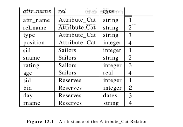
An elegant aspect of a relational DBMS is that the system catalog is itself a collection of tables. For example, we might store information about the attributes of tables in a catalog table called Attribute_Cat:
Attribute_Cat( attr_name: string, rel_name: string,
                type: string, position: integer)
Suppose that the database contains the two tables that we introduced at the begining of this chapter:
Sailors(sid: integer, sname: string, rating: integer, age: real)
Reserves(sid: integer, bid: integer, day: dates, mame: string)
Figure 12.1 shows the tuples in the Attribute_Cat table that describe the attributes of these two tables. Note that in addition to the tuples describing Sailors and Reserves, other tuples (the first four listed) describe the four attributes of the Attribute_Cat table itself. These other tuples illustrate an important Point: the catalog tables describe all the tables in the database, including the catalog tables themselves. When information about a table is needed, it is obtained from the system catalog. Of course, at the implementation level, whenever the DBMS needs to find the schema of a catalog table, the code that retrieves this information must be handled specially. (Otherwise, the code has to retrieve this information from the catalog tables without, presumably, knowing the schema of the catalog tables.)
The fact that the system catalog is also a collection of tables is very useful. For example, catalog tables can be queried just like any other table, using the query language of the DBMS. Further, all the techniques available for implementing and managing tables apply directly to catalog tables. The choice of catalog tables and their schema, is not unique and is made by the implementor of the DBMS. Real systems vary in their catalog schema design, but the catalog is always implemented as a collection of tables, and it essentially describes all the data stored in the database.
Introduction to Operator Evaluation
Several alternative algorithms are available for implementing each relational operator, and for most operators no algorithm is universally superior. Several factors influence which algorithm performs best, including the sizes of the tables involved, existing indexes and sort orders, the size of the available buffer pool, and the buffer replacement policy.
Three Common Techniques
The algorithms for various relational operators actually have a lot in common. A few simple techniques are used to develop algorithms for each operator:
- Indexing: If a selection or join condition is specified, use an index to examine just the tuples that satisfy the condition.
- Iteration: Examine all tuples in an input table, one after the other. If we need only a few fields from each tuple and there is an index whose key contains all these fields, instead of examining data tuples, we can scan all index data entries. (Scanning all data entries sequentially makes no use of the index’s hash–or tree-based search structure; in a tree index, for example, we would simply examine all leaf pages in sequence.)
- Partitioning: By partitioning tuples on a sort key, we can often decompose an operation into a less expensive collection of operations on partitions. Sorting and hashing are two commonly used partitioning techniques.
Access Paths
An access path is a way of retrieving tuples from a table and consists of either (1) a file scan or (2) an index plus a matching selection condition. Every relational operator accepts one or more tables as input, and the access methods used to retrieve tuples contribute significantly to the cost of the operator. Consider a simple selection that is a conjunction of conditions of the form attr op value, where op is one of the comparison operators $<, \leq, =, \neq, \geq, or >$. Such selections are said to be in conjunctive normal form (CNF), and each condition is called a conjunct. Intuitively, an index matches a selection condition if the index can be used to retrieve just the tuples that satisfy the condition.
- A hash index matches a CNF selection if there is a term of the form attribute=value in the selection for each attribute in the index’s search key.
- A tree index matches a CNF selection if there is a term of the form attribute op value for each attribute in a prefix of the index’s search key. ((a)) and (a,b) are prefixes of key (a,b,e), but (a,e) and (b,e) are not.) Note that op can be any comparison; it is not restricted to be equality as it is for matching selections on a hash index.
An index can match some subset of the conjuncts in a selection condition (in CNP), even though it does not match the entire condition. We refer to the conjuncts that the index matches as the primary conjuncts in the selection.
The following examples illustrate access paths.
- If we have a hash index H on the search key (rname, bid, sid), we can use the index to retrieve just the Sailors tuples that satisfy the condition rname=’Joe’ $\wedge$ bid=5 $\wedge$ sid=3. The index matches the entire condition rname= ‘Joe’ $\wedge$ bid=5 $\wedge$ sid= 3. On the other hand, if the selection condition is rname= ‘Joe’ $\wedge$ bid=5, or some condition on date, this index does not match. That is, it cannot be used to retrieve just the tuples that satisfy these conditions. In contrast, if the index were a B+ tree, it would match both rname= ‘Joe’ $\wedge$ bid=5 $\wedge$ sid=3 and mame=’Joe’ $\wedge$ bid=5. However, it would not match bid=5 $\wedge$ sid=8 (since tuples are sorted primarily by rname).
- If we have an index (hash or tree) on the search key (bid,sid) and the selection condition rname= ‘Joe’ $\wedge$ bid=5 $\wedge$ sid=3, we can use the index to retrieve tuples that satisfy bid=5 $\wedge$ sid=3; these are the primary conjuncts. The fraction of tuples that satisfy these conjuncts (and whether the index is clustered) determines the number of pages that are retrieved. The additional condition on rname must then be applied to each retrieved tuple and will eliminate some of the retrieved tuples from the result.
- If we have an index on the search key (bid,sid) and we also have a B+ tree index on day, the selection condition $day < 8/9/2002 \wedge bid=5 \wedge sid=3$ offers us a choice. Both indexes match (part of) the selection condition, and we can use either to retrieve Reserves tuples. Whichever index we use, the conjuncts in the selection condition that are not matched by the index (e.g., bid=5 $\wedge$ sid=3 if we use the B+ tree index on day) must be checked for each retrieved tuple.
The selectivity of an access path is the number of pages retrieved (index pages plus data pages) if we use this access path to retrieve all desired tuples. If a table contains an index that matches a given selection, there are at least two access paths: the index and a scan of the data file. Sometimes, of course, we can scan the index itself (rather than scanning the data file or using the index to probe the file), giving us a third access path.
The most selective access path is the one that retrieves the fewest pages; using the most selective access path minimizes the cost of data retrieval. The selectivity of an access path depends on the primary conjuncts in the selection condition (with respect to the index involved). Each conjunct acts as a filter on the table. The fraction of tuples in the table that satisfy a given conjunct is called the reduction factor. When there are several primary conjuncts, the fraction of tuples that satisfy all of them can be approximated by the product of their reduction factors; this effectively treats them as independent filters, and while they may not actually be independent, the approximation is widely used in practice.
Supose we have a hash index H on Sailors with search key (rname,bid,sid), and we are given the selection condition rname=’Joe’ $\wedge$ bid=5 $\wedge$ sid=3. We can use the index to retrieve tuples that satisfy all three conjuncts. The catalog contains the number of distinct key values, N keys(H), in the hash index, as well as the number of pages, N Pages, in the Sailors table. The fraction of pages satisfying the primary conjuncts is N pages(Sailors).
If the index has search key (bid,sid) , the primary conjuncts are bid=5 $\wedge$ sid=3. If we know the number of distinct values in the bid column, we can estimate the reduction factor for the first conjunct. This information is available in the catalog if there is an index with bid as the search key; if not, optimizers typically use a default value such as 1/10. Multiplying the reduction factors for bid=5 and sid=3 gives us (under the simplifying independence assumption) the fraction of tuples retrieved; if the index is clustered, this is also the fraction of pages retrieved. If the index is not clustered, each retrieved tuple could be on a different page.
Algorithm For Relational Operations
The selection operation is a simple retrieval of tuples from a table, and its implementation is essentially covered in our discussion of access paths. To summarize, given a selection of the form $\sigma_{R.attr}$ op value(R), if there is no index on R.attr, we have to scan R. If one or more indexes on R match the selection, we can use the index to retrieve matching tuples, and apply any remaining selection conditions to further restrict the result set. As an example, consider a selection of the form rname < ‘C%’ on the Reserves table. Assuming that names are uniformly distributed with respect to the initial letter, for simplicity, we estimate that roughly 10% of Reserves tuples are in the result. This is a total of 10,000 tuples, or 100 pages. If we have a clustered B+ tree index on the rname field of Reserves, we can retrieve the qualifying tuples with 100 I/Os (plus a few I/Os to traverse from the root to the appropriate leaf page to start the scan). However, if the index is unclustered , we could have up to 10,000 I/Os in the worst case, since each tuple could cause us to read a page. As a rule of thumb, it is probably cheaper to simply scan the entire table (instead of using an unclustered index) if over 5% of the tuples are to be retrieved.
The projection operation requires us to drop certain fields of the input, which is easy to do. The expensive aspect of the operation is to ensure that no duplicates appear in the result. For example, if we only want the sid and bid fields from Reserves, we could have duplicates if a sailor has reserved a given boat on several days. If duplicates need not be eliminated (e.g., the DISTINCT keyword is not included in the SELECT clause), projection consists of simply retrieving a subset of fields from each tuple of the input table. This can be accomplished by simple iteration on either the table or an index whose key contains all necessary fields. (Note that we do not care whether the index is clustered, since the values we want are in the data entries of the index itself!) If we have to eliminate duplicates, we typically have to use partitioning. Suppose we want to obtain (sid, bid) by projecting from Reserves. We can partition by (1) scanning Reserves to obtain (sid, bid) pairs and (2) sorting these pairs using (sid, bid) as the sort key. We can then scan the sorted pairs and easily discard duplicates, which are now adjacent. Sorting large disk-resident datasets is a very important operation in database systems. Sorting a table typically requires two or three passes, each of which reads and writes the entire table. The projection operation can be optimized by combining the initial scan of Reserves with the scan in the first pass of sorting. Similarly, the scanning of sorted pairs can be combined with the last pass of sorting. With such an optimized implemention, projection with duplicate elimination requires (1) a first pass in which the entire table is scanned, and only pairs (sid, bid) are written out, and (2) a final pass in which all pairs are scanned, but only one copy of each pair is written out. In addition, there might be an intermediate pass in which all pairs are read from and written to disk. The availability of appropriate indexes can lead to less expensive plans than sorting for duplicate elimination. If we have an index whose search key contains all the fields retained by the projection, we can sort the data entries in the index, rather than the data records themselves. If all the retained attributes appear in a prefix of the search key for a clustered index, we can do even better; we can simply retrieve data entries using the index, and duplicates are easily detected since they are adjacent. These plans are further examples of index-only evaluation strategies.
Joins are expensive operations and very common. Therefore, they have been widely studied, and systems typically support several algorithms to carry out joins. Consider the join of Reserves and Sailors, with the join condition Reserves.sid = Sailors.sid. Suppose that one of the tables, say Sailors, has an index on the sid column. We can scan Reserves and, for each tuple, use the index to probe Sailors for matching tuples. This approach is called index nested loops join. Suppose that we have a hash-based index using Alternative (2) on the sid attribute of Sailors and that it takes about 1.2 I/Os on average to retrieve the appropriate page of the index. Since sid is a key for Sailors, we have at most one matching tuple, Indeed, sid in Reserves is a foreign key referring to Sailors, and therefore we have exactly one matching Sailors tuple for each Reserves tuple, Let us consider the cost of scanning Reserves and using the index to retrieve the matching Sailors tuple for each Reserves tuple. The cost of scanning Reserves is 1000. There are 100 * 1000 tuples in Reserves. For each of these tuples, retrieving the index page containing the rid of the matching Sailors tuple costs 1.2 I/Os (on average); in addition, we have to retrieve the Sailors page containing the qualifying tuple, Therefore, we have 100,000 * (1 + 1.2) I/Os to retrieve matching Sailors tuples. The total cost is 221,000 I/Os. If we do not have an index that matches the join condition on either table, we cannot use index nested loops, In this case, we can sort both tables on the join column, and then scan them to find matches. This is called sort-merge join. Assuming that we can sort Reserves in two passes, and Sailors in two passes as well, let us consider the cost of sort-merge join. Consider the join of the tables Reserves and Sailors. Because we read and write Reserves in each pass, the sorting cost is 2 * 2 * 1000 = 4000 I/Os. Similarly, we can sort Sailors at a cost of 2 * 2 * 500 = 2000 I/Os. In addition, the second phase of the sort-merge join algorithm requires an additional scan of both tables. Thus the total cost is 4000 + 2000 + 1000 + 500 = 7500 I/Os. Observe that the cost of sort-merge join, which does not require a pre-existing index, is lower than the cost of index nested loops join, In addition, the result of the sort-merge join is sorted on the join column(s). Other join algorithms that do not rely on an existing index and are often cheaper than index nested loops join are also known. Given this, why consider index nested loops at all? Index nested loops has the nice property that it is incremental. The cost of our example join is incremental in the number of Reserves tuples that we process. Therefore, if some additional selection in the query allows us to consider only a small subset of Reserves tuples, we can avoid computing the join of Reserves and Sailors in its entirety. For instance, suppose that we only want the result of the join for boat 101, and there are very few such reservations. for each such Reserves tuple, we probe Sailors, and we are done. If we use sort-merge join, on the other hand, we have to scan the entire Sailors table at least once, and the cost of this step alone is likely to be much higher than the entire cost of index nested loops join. Observe that the choice of index nested loops join is based on considering the query as a whole, including the extra selection all Reserves, rather than just the join operation by itself. This leads us to our next topic, query optimization, which is the process of finding a good plan for an entire query.
Introduction to Query Optimization
Query optimization is one of the most important tasks of a relational DBMS. One of the strengths of relational query languages is the wide variety of ways in which a user can express and thus the system can evaluate a query. Although this flexibility makes it easy to write queries, good performance relies greatly on the quality of the query optimizer–a given query can be evaluated in many ways, and the difference in cost between the best and worst plans may be several orders of magnitude. Realistically, we cannot expect to always find the best plan, but we expect to consistently find a plan that is quite good. Queries are parsed and then presented to a query optimizer, which is responsible for identifying an efficient execution plan. The optimizer generates alternative plans and chooses the plan with the least estimated cost.
Query Evaluation Plans
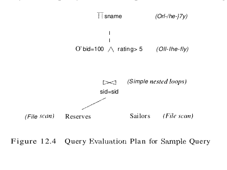
A query evaluation plan (or simply plan) consists of an extended relational algebra tree, with additional annotations at each node indicating the access methods to use for each table and the implementation method to use for each relational operator. Consider the following SQL query:
SELECT S.sname
FROM Reserves R, Sailors S
WHERE R.sid = S.sid
AND R.bid = 100 AND S.rating > 5
This query can be expressed in relational algebra as follows:
$\pi_{\text {sname }}\left(\sigma_{\text {bid }=100 \wedge \text { rating }>5}\left(\text { Reserves } \bowtie_{\text {sid }=\text { sid }} \text { Sailors }\right)\right)$
This expression is shown in the form of a tree in Figure 12.3. The algebra expression partially specifies how to evaluate the query–we first compute the natural join of Reserves and Sailors, then perform the selections, and finally project the sname field.

To obtain a fully specified evaluation plan, we must decide on an implementation for each of the algebra operations involved. For example, we can use a page-oriented simple nested loops join with Reserves as the outer table and apply selections and projections to each tuple in the result of the join as it is produced; the result of the join before the selections and projections is never stored in its entirety. This query evaluation plan is shown in Figure 12.4.
Multi-operator Queries: Pipelined Evaluation
When a query is composed of several operators, the result of one operator is sometimes pipelined to another operator without creating a temporary table to hold the intermediate result. The plan in Figure 12.4 pipelines the output of the join of Sailors and Reserves into the selections and projections that follow. Pipelining the output of an operator into the next operator saves the cost of writing out the intermediate result and reading it back in, and the cost savings can be significant. If the output of an operator is saved in a temporary table for processing by the next operator, we say that the tuples are materialized. Pipelined evaluation has lower overhead costs than materialization and is chosen whenever the algorithm for the operator evaluation permits it. There are many opportunities for pipelining in typical query plans, even simple plans that involve only selections. Consider a selection query in which only part of the selection condition matches an index. We can think of such a query as containing two instances of the selection operator: The first contains the primary, or matching, part of the original selection condition, and the second contains the rest of the selection condition. We can evaluate such a query by applying the primary selection and writing the result to a temporary table and then applying the second selection to the temporary table. In contrast, a pipelined evaluation consists of applying the second selection to each tuple in the result of the primary selection as it is produced and adding tuples that qualify to the final result. When the input table to a unary operator (e.g., selection or projection) is pipelined into it, we sometimes say that the operator is applied on-the-fly. As a second and more general example, consider a join of the form $(A \bowtie B) \bowtie C$, shown in Figure 12.5 as a tree of join operations.

Both joins can be evaluated in pipelined fashion using some version of a nested loops join. Conceptually, the evaluation is initiated from the root, and the node joining A and B produces tuples as and when they are requested by its parent node. When the root node gets a page of tuples from its left child (the outer table), all the matching inner tuples are retrieved (using either an index or a scan) and joined with matching outer tuples; the current page of outer tuples is then discarded. A request is then made to the left child for the next page of tuples, and the process is repeated. Pipelined evaluation is thus a control strategy governing the rate at which different joins in the plan proceed. It has the great virtue of not writing the result of intermediate joins to a temporary file because the results are produced, consumed, and discarded one page at a time.
The Iterator Interface
A query evaluation plan is a tree of relational operators and is executed by calling the operators in some (possibly interleaved) order. Each operator has one or more inputs and an output, which are also nodes in the plan, and tuples must be passsed between operators according to the plan’s tree structure.
To simplify the code responsible for coordinating the execution of a plan, the relational operators that form the nodes of a plan tree (which is to be evaluated using pipelining) typically support a uniform iterator interface, hiding the internal implementation details of each operator.
The iterator interface supports pipelining of results naturally: the decision to pipeline or materialize input tuples is encapsulated in the operator-specific code that processes input tuples. If the algorithm implemented for the operator allows input tuples to be processed completely when they are received, input tuples are not materialized and the evaluation is pipelined. If the algorithm examines the same input tuples several times, they are materialized.
Alternative Plans: A Motivating Example
Consider the example query above. Let us consider the cost of evaluating the plan shown in Figure 12.4. We ignore the cost of writing out the final result since this is common to all algorithms, and does not affect their relative costs. The cost of the join is 1000 + 1000 * 500 = 501,000 page I/Os. The selections and the projection are done on-the-fly and do not incur additional I/Os. The total cost of this plan is therefore 501,000 page I/Os. This plan is admittedly naive; however, it is possible to be even more naive by treating the join as a cross-product followed by a selection. We now consider several alternative plans for evaluating this query.
Pushing Selections
A join is a relatively expensive operation, and a good heuristic is to reduce the sizes of the tables to be joined as much as possible. One approach is to apply selections early; if a selection operator appears after a join operator, it is worth examining whether the selection can be ‘pushed’ ahead of the join. As an example, the selection bid = 1 involves only the attributes of Reserves and can be applied to Reserves before the join. Similarly, the selection rating > 5 involves only attributes of Sailors and can be applied to Sailors before the join. Let us suppose that the selections are performed using a simple file scan, that the result of each selection is written to a temporary table on disk, and that the temporary tables are then joined using a sort-merge join. The resulting query evaluation plan is shown in Figure 12.6.

Let us assume that five buffer pages are available and estimate the cost of this query evaluation plan. (It is likely that more buffer pages are available in practice. We chose a small number simply for illustration in this example.) The cost of applying bid = 100 to Reserves is the cost of scanning Reserves (1000 pages) plus the cost of writing the result to a temporary table, say T1. (Note that the cost of writing the temporary table cannot be ignored-we can ignore only the cost of writing out the final result of the query, which is the only component of the cost that is the same for all plans.) To estimate the size of T1, we require additional information. For example, if we assume that the maximum number of reservations of a given boat is one, just one tuple appears in the result. Alternatively, if we know that there are 100 boats, we can assume that reservations are spread out uniformly across all boats and estimate the number of pages in T1 to be 10. For concreteness, assume that the number of pages in T1 is indeed 10. The cost of applying rating > 5 to Sailors is the cost of scanning Sailors (500 pages) plus the cost of writing out the result to a temporary table, say, T2. If we assume that ratings are uniformly distributed over the range 1 to 10, we can approximately estimate the size of T2 as 250 pages. To do a sort-merge join of T1 and T2, let us assume that a straightforward implementation is used in which the two tables are first completely sorted and then merged. Since five buffer pages are available, we can sort T1 (which has 10 pages) in two passes. Two runs of five pages each are produced in the first pass and these are merged in the second pass. In each pass, we read and write 10 pages; thus, the cost of sorting T1 is 2 * 2 * 10 = 40 page I/Os. We need four passes to sort T2, which has 250 pages. The cost is 2 * 4 * 250 = 2000 page I/Os. To merge the sorted versions of T1 and T2, we need to scan these tables, and the cost of this step is 10 + 250 = 260. The final projection is done on-the-fly, and by convention we ignore the cost of writing the final result. The total cost of the plan shown in Figure 12.6 is the sum of the cost of the selection (1000+10+500+250 = 1760) and the cost of the join (40+2000+260 = 2300, that is, 4060 page I/Os. Sort-merge join is one of several join methods. We may be able to reduce the cost of this plan by choosing a different join method. As an alternative, suppose that we used block nested loops join instead of sort-merge join. Using T1 as the outer table, for every three-page block of T1, we scan all of T2; thus, we scan T2 four times. The cost of the join is therefore the cost of scanning T1 (10) plus the cost of scanning T2 (4 * 250 = 1000). The cost of the plan is now 1760 + 1010 = 2770 page I/Os. A further refinement is to push the projection, just like we pushed the selections past the join. Observe that only the sid attribute of T1 and the sid and sname attributes of T2 are really required. As we scan Reserves and Sailors to do the selections, we could also eliminate unwanted columns. This on-the-fly projection reduces the sizes of the temporary tables T1 and T2. The reduction in the size of T1 is substantial because only an integer field is retained. In fact, T1 now fits within three buffer pages, and we can perform a block nested loops join with a single scan of T2. The cost of the join step drops to under 250 page I/Os, and the total cost of the plan drops to about 2000 I/Os.
Using Indexes
If indexes are available on the Reserves and Sailors tables, even better query evaluation plans may be available. For example, suppose that we have a clustered static hash index on the bid field of Reserves and another hash index on the sid field of Sailors. We can then use the query evaluation plan shown in Figure 12.7.
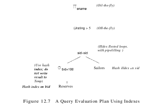
The selection bid = 100 is performed on Reserves by using the hash index on bid to retrieve only matching tuples. As before, if we know that 100 boats are available and assume that reservations are spread out uniformly across all boats, we can estimate the number of selected tuples to be 100000/100 = 1000. Since the index on bid is clustered, these 1000 tuples appear consecutively within the same bucket; therefore, the cost is 10 page I/Os. For each selected tuple, we retrieve matching Sailors tuples using the hash index on the sid field; selected Reserves tuples are not materialized and the join is pipelined. For each tuple in the result of the join, we perform the selection rating > 5 and the projection of sname on-the-fly. There are several important points to note here:
- Since the result of the selection on Reserves is not materialized, the optimization of projecting out fields that are not needed subsequently is unnecessary (and is not used in the plan shown in Figure 12.7).
- The join field sid is a key for Sailors. Therefore, at most one Sailors tuple matches a given Reserves tuple. The cost of retrieving this matching tuple depends on whether the directory of the hash index on the sid column of Sailors fits in memory and on the presence of overflow pages (if any). However, the cost does not depend on whether this index is clustered because there is at most one matching Sailors tuple and requests for Sailors tuples are made in random order by sid (because Reserves tuples are retrieved by bid and are therefore considered in random order by sid). For a hash index, 1.2 page I/Os (on average) is a good estimate of the cost for retrieving a data entry. Assuming that the sid hash index on Sailors uses Alternative (1) for data entries, 1.2 I/Os is the cost to retrieve a matching Sailors tuple (and if one of the other two alternatives is used, the cost would be 2.2 I/Os).
- We have chosen not to push the selection rating > 5 ahead of the join, and there is an important reason for this decision. If we performed the selection before the join, the selection would involve scanning Sailors, assuming that no index is available on the rating field of Sailors. Further, whether or not such an index is available, once we apply such a selection, we have no index on the sid field of the result of the selection (unless we choose to build such an index solely for the sake of the subsequent join). Thus, pushing selections ahead of joins is a good heuristic, but not always the best strategy. Typically, as in this example, the existence of useful indexes is the reason a selection is not pushed. (Otherwise, selections are pushed.)
Let us estimate the cost of the plan shown in Figure 12.7. The selection of Reserves tuples costs 10 I/Os, as we saw earlier. There are 1000 such tuples, and for each, the cost of finding the matching Sailors tuple is 1.2 I/Os, on average. The cost of this step (the join) is therefore 1200 I/Os. All remaining selections and projections are performed on-the-fly. The total cost of the plan is 1210 I/Os.
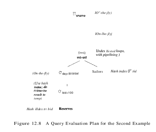
As noted earlier, this plan does not utilize clustering of the Sailors index. The plan can be further refined if the index on the sid field of Sailors is clustered. Suppose we materialize the result of performing the selection bi = 100 on Reserves and sort this temporary table. This table contains 10 pages. Selecting the tuples costs 10 page I/Os (as before), writing out the result to a temporary table costs another 10 I/Os, and with five buffer pages, sorting this temporary costs 2 * 2 * 10 = 40 I/Os. (The cost of this step is reduced if we push the projection on sid. The sid column of materialized Reserves tuples requires only three pages and can be sorted in memory with five buffer pages.) The selected Reserves tuples can now be retrieved in order by sid. If a sailor has reserved the same boat many times, all corresponding Reserves tuples are now retrieved consecutively; the matching Sailors tuple will be found in the buffer pool on all but the first request for it. This improved plan also demonstrates that pipelining is not always the best strategy. The combination of pushing selections and using indexes illustrated by this plan is very powerful. If the selected tuples from the outer table join with a single inner tuple, the join operation may become trivial, and the performance gains with respect to the naive plan in Figure 12.6 are even more dramatic. The following variant of our example query illustrates this situation:
SELECT S.sname
FROM Reserves R, Sailors S
WHERE Rsid = S.sid
AND R.bid = 100 AND S.rating
AND Rday = '8/9/2002'
A slight variant of the plan shown in Figure 12.7, designed to answer this query, is shown in Figure 12.8. The selection day = ‘8/9/2002’ is applied on-the-fly to the result of the selection bid = 100 on the Reserves table. Suppose that bid and day form a key for Reserves. Let us estimate the cost of the plan shown in Figure 12.8. The selection bid = 100 costs 10 page I/Os, as before, and the additional selection day = ‘8/9/2002’ is applied on-the-fly, eliminating all but (at most) one Reserves tuple. There is at most one matching Sailors tuple, and this is retrieved in 1.2 I/Os (an average value). The selection on rating and the projection on sname are then applied on-the-fly at no additional cost. The total cost of the plan in Figure 12.8 is thus about 11 I/Os. In contrast, if we modify the naive plan in Figure 12.6 to perform the additional selection on day together with the selection bid = 100, the cost remains at 501,000 I/Os.
What a Typical Optimizer Does
A relational query optimizer uses relational algebra equivalences to identify many equivalent expressions for a given query. For each such equivalent version of the query, all available implementation techniques are considered for the relational operators involved, thereby generating several alternative query evaluation plans. The optimizer estimates the cost of each such plan and chooses the one with the lowest estimated cost.
Two relational algebra expressions over the same set of input tables are said to be equivalent if they produce the same result on all instances of the input tables. Relational algebra equivalences playa central role in identifying alternative plans.
Consider a basic SQL query consisting of a SELECT clause, a FROM clause, and a WHERE clause, This is easily represented as an algebra expression; the fields mentioned in the SELECT are projected from the cross-product of tables in the FROM clause, after applying the selections in the WHERE clause. The use of equivalences enable us to convert this initial representation into equivalent expressions. In particular:
- Selections and cross-products can be combined into joins.
- Joins can be extensively reordered.
- Selections and projections, which reduce the size of the input, can be “pushed” ahead of joins.
Left-Deep Plans
Consider a query of the form $A \bowtie B \bowtie C \bowtie D$; that is, the natural join of four tables. Three relational algebra operator trees that are equivalent to this query (based on algebra equivalences) are shown in Figure 12.9. By convention, the left child of a join node is the outer table and the right child is the inner table. By adding details such as the join method for each join node, it is straightforward to obtain several query evaluation plans from these trees.
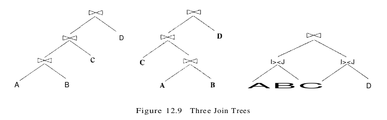
The first two trees in Figure 12.9 are examples of linear trees. In a linear tree, at least one child of a join node is a base table. The first tree is an example of a left-deep tree–the right child of each join node is a base table. The third tree is an example of a non-linear or bushy tree. Optimizers typically use a dynamic-programming approach to efficiently search the class of a left-deep plans. The second and third kinds of trees are therefore never considered. Intuitively, the first tree represents a plan in which we join A and B first, then join the result with C, then join the result with D. There are 23 other left-deep plans that differ only in the order that tables are joined. If any of these plans has selection and projection conditions other than the joins themselves, these conditions are applied as early as possible (consitent with algebra equivalences) given the choice of a join order for the tables. Of course, this decision rules out many alternative plans that may cost less than the best plan using a left-deep tree; we have to live with the fact that the optimizer will never find such plans. There are two main reasons for this decision to concentrate on left-deep plans, or plans based on left-deep trees:
- As the number of joins increases, the number of alternative plans increases rapidly and it becomes necessary to prune the space of alternative plans.
- Left-deep trees allow us to generate all fully pipelined plans; that is, plans in which all joins are evaluated using pipelining. (Inner tables must always be materialized because we must examine the entire inner table for each tuple of the outer table. So, a plan in which an inner table is the result of a join forces us to materialize the result of that join.)
Estimating the Cost of a Plan
The cost of a plan is the sum of costs for the operators it contains. The cost of individual relational operators in the plan is estimated using information, obtained from the system catalog, about properties (e.g., size, sort order) of their input tables. If we focus on the metric of I/O costs, the cost of a plan can be broken down into three parts: (1) reading the input tables (possibly multiple times in the case of some join and sorting algorithms), (2) writing intermediate tables, and (possibly) (3) sorting the final result (if the query specifies duplicate elimination or an output order). The third part is common to all plans (unless one of the plans happens to produce output in the required order), and, in the common case that a fully-pipelined plan is chosen, no intermediate tables are written. Thus, the cost for a fully-pipelined plan is dominated by part (1). This cost depends greatly on the access paths used to read input tables; of course, access paths that are used repeatedly to retrieve matching tuples in a join algorithm are especially important. For plans that are not fully pipelined, the cost of materializing temporary tables can be significant. The cost of materializing an intermediate result depends on its size, and the size also infiuences the cost of the operator for which the temporary is an input table. The number of tuples in the result of a selection is estimated by multiplying the input size by the reduction factor for the selection conditions. The number of tuples in the result of a projection is the same as the input, assuming that duplicates are not eliminated; of course, each result tuple is smaller since it contains fewer fields. The result size for a join can be estimated by multiplying the maximum result size, which is the product of the input table sizes, by the reduction factor of the join condition.