- Data on External Storage
- File Organizations and Indexing
- Index Data Structures
- Comparison of File Organizations
- Indexes and Performance Tuning
The basic abstraction of data in a DBMS is a collection of records, or a file, and each file consists of one or more pages. A file organization is a method of arranging the records in a file when the file is stored on disk. Each file organization makes certain operations efficient but other operations expensive.
Consider a file of employee records, each containing age, name, and sal fields, which we use as a running example in this chapter. If we want to retrieve employee records in order of increasing age, sorting the file by age is a good file organization, but the sort order is expensive to maintain if the file is frequently modified. Further, we are often interested in supporting more than one operation on a given collection of records. In our example, we may also want to retrieve all employees who make more than $5000. We have to scan the entire file to find such employee records. A technique called indexing can help when we have to access a collection of records in multiple ways, in addition to efficiently supporting various kinds of selection.
Data on External Storage
A DBMS stores vast quantities of data, and the data must persist across program executions. Therefore, data is stored on external storage devices such as disks and tapes, and fetched into main memory as needed for processing. The unit of information read from or written to disk is a page. The size of a page is a DBMS parameter, and typical values are 4KB or 8KB.
The following points are important to keep in mind:
- Disks are the most important external storage devices. They allow us to retrieve any page at a (more or less) fixed cost per page. However, if we read several pages in the order that they are stored physically, the cost can be much less than the cost of reading the same pages in a random order.
- Tapes are sequential access devices and force us to read data one page after the other. They are mostly used to archive data that is not needed on a regular basis.
- Each record in a file has a unique identifier called a record id, or rid for short. An rid has the property that we can identify the disk address of the page containing the record by using the rid.
Data is read into memory for processing, and written to disk for persistent storage, by a layer of software called the buffer manager. When the files and access methods layer (which we often refer to as just the file layer) needs to process a page, it asks the buffer manager to fetch the page, specifying the page’s rid. The buffer manager fetches the page from disk if it is not already in memory.
Space on disk is managed by the disk space manager. When the files and access methods layer needs additional space to hold new records in a file, it asks the disk space manager to allocate an additional disk page for the file; it also informs the disk space manager when it no longer needs one of its disk pages. The disk space manager keeps track of the pages in use by the file layer; if a page is freed by the file layer, the space manager tracks this, and reuses the space if the file layer requests a new page later on.
File Organizations and Indexing
The file of records is an important abstraction in a DBMS, and is implemented by the files and access methods layer of the code. A file can be created, destroyed, and have records inserted into and deleted from it. It also supports scans; a scan operation allows us to step through all the records in the file one at a time. A relation is typically stored as a file of records.
The file layer stores the records in a file in a collection of disk pages. It keeps track of pages allocated to each file, and as records are inserted into and deleted from the file, it also tracks available space within pages allocated to the file.
The simplest file structure is an unordered file, or heap file. Records in a heap file are stored in random order across the pages of the file. A heap file organization supports retrieval of all records, or retrieval of a particular record specified by its rid; the file manager must keep track of the pages allocated for the file.
An index is a data structure that organizes data records on disk to optimize certain kinds of retrieval operations. An index allows us to efficiently retrieve all records that satisfy search conditions on the search key fields of the index. We can also create additional indexes on a given collection of data records, each with a different search key, to speed up search operations that are not efficiently supported by the file organization used to store the data records.
Consider our example of employee records. We can store the records in a file organized as an index on employee age; this is an alternative to sorting the file by age. Additionally, we can create an auxiliary index file based on salary, to speed up queries involving salary. The first file contains employee records, and the second contains records that allow us to locate employee records satisfying a query on salary.
We use the term data entry to refer to the records stored in an index file. A data entry with search key value k, denoted as k*, contains enough information to locate (one or more) data records with search key value k. We can efficiently search an index to find the desired data entries, and then use these to obtain data records (if these are distinct from data entries).
There are three main alternatives for what to store as a data entry in an index:
- A data entry k* is an actual data record (with search key value k).
- A data entry is a (k, rid) pair, where rid is the record id of a data record with search key value k.
- A data entry is a (k. rid-list) pair, where rid-list is a list of record ids of data records with search key value k.
Clustered Indexes
When a file is organized so that the ordering of data records is the same as or close to the ordering of data entries in some index, we say that the index is clustered; otherwise, it is an unclustered index. An index that uses Alternative (1) is clustered, by definition. An index that uses Alternative (2) or (3) can be a clustered index only if the data records are sorted on the search key field. Otherwise, the order of the data records is random, defined purely by their physical order, and there is no reasonable way to arrange the data entries in the index in the same order.
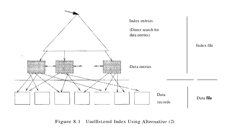
The cost of using an index to answer a range search query can vary tremendously based on whether the index is clustered. If the index is clustered, i.e., we are using the search key of a clustered file, the rids in qualifying data entries point to a contiguous collection of records, and we need to retrieve only a few data pages. If the index is unclustered, each qualifying data entry could contain a rid that points to a distinct data page, leading to as many data page I/Os as the number of data entries that match the range selection, as illustrated in Figure 8.1.
Primary and Secondary Indexes
An index on a set of fields that includes the primary key is called a primary index; other indexes are called secondary indexes. (The terms primary index and secondary index are sometimes used with a different meaning: An index that uses Alternative (1) is called a primary index, and one that uses Alternatives (2) or (3) is called a secondary index. We will be consistent with the definitions presented earlier, but the reader should be aware of this lack of standard terminology in the literature.)
Two data entries are said to be duplicates if they have the same value for the search key field associated with the index. A primary index is guaranteed not to contain duplicates, but an index on other (collections of) fields can contain duplicates. In general, a secondary index contains duplicates. If we know that no duplicates exist, that is, we know that the search key contains some candidate key, we call the index a unique index.
Index Data Structures
One way to organize data entries is to hash data entries on the search key. Another way to organize data entries is to build a tree-like data structure that directs a search for data entries. We note that the choice of hash or tree indexing techniques can be combined with any of the three alternatives for data entries.
Hash-Based Indexing
We can organize records using a technique called hashing to quickly find records that have a given search key value. For example, if the file of employee records is hashed on the name field, we can retrieve all records about Joe. In this approach, the records in a file are grouped in buckets, where a bucket consists of a primary page and, possibly, additional pages linked in a chain. The bucket to which a record belongs can be determined by applying a special function, called a hash function, to the search key. Given a bucket number, a hash-based index structure allows us to retrieve the primary page for the bucket in one or two disk I/Os. On inserts, the record is inserted into the appropriate bucket, with ‘overflow’ pages allocated as necessary. To search for a record with a given search key value, we apply the hash function to identify the bucket to which such records belong and look at all pages in that bucket. If we do not have the search key value for the record, for example, the index is based on sal and we want records with a given age value, we have to scan all pages in the file.
Hash indexing is illustrated in Figure 8.2, where the data is stored in a file that is hashed on age; the data entries in this first index file are the actual data records. Applying the hash function to the age field identifies the page that the record belongs to. The hash function h for this example is quite simple; it converts the search key value to its binary representation and uses the two least significant bits as the bucket identifier. Figure 8.2 also shows an index with search key sal that contains (sal, rid) pairs as data entries. The rid (short for record id) component of a data entry in this second index is a pointer to a record with search key value sal (and is shown in the figure as an arrow pointing to the data record). Note that the search key for an index can be any sequence of one or more fields, and it need not uniquely identify records. For example, in the salary index, two data entries have the same search key value 6003.

Tree-Based Indexing
Figure 8.3 shows the employee records from Figure 8.2, this time organized in a tree-structured index with search key age. Each node in this figure (e.g., nodes labeled A, B, L1, L2) is a physical page, and retrieving a node involves a disk I/O. The lowest level of the tree, called the leaf level, contains the data entries; In our example, these are employee records. To illustrate the ideas better, we have drawn Figure 8.3 as if there were additional employee records, some with age less than 22 and some with age greater than 50 (the lowest and highest age values that appear in Figure 8.2). Additional records with age less than 22 would appear in leaf pages to the left page L1, and records with age greater than 50 would appear in leaf pages to the right of page L3.

This structure allows us to efficiently locate all data entries with search key values in a desired range. All searches begin at the topmost node, called the root, and the contents of pages in non-leaf levels direct searches to the correct leaf page. Non-leaf pages contain node pointers separated by search key values. The node pointer to the left of a key value k points to a subtree that contains only data entries less than k. The node pointer to the right of a key value k points to a subtree that contains only data entries greater than or equal to k.
Comparison of File Organizations
We now compare the costs of some simple operations for several basic file organizations on a collection of employee records. We assume that the files and indexes are organized according to the composite search key (age, sal), and that all selection operations are specified on these fields. The organizations that we consider are the following:
- File of randomly ordered employee records, or heap file.
- File of employee records sorted on (age, sal).
- Clustered B+ tree file with search key (age, sal).
- Heap file with an unclustered B+ tree index on (age, sal).
- Heap file with an unclustered hash index on (age, sal).
Note that even if the data file is sorted, an index whose search key differs from the sort order behaves like an index on a heap file. The operations we consider are these:
- Scan: Fetch all records in the file. The pages in the file must be fetched from disk into the buffer pool. There is also a CPU overhead per record for locating the record on the page (in the pool).
- Search with Equality Selection: Fetch all records that satisfy an equality selection; for example, “Find the employee record for the employee with age 23 and sal 50.” Pages that contain qualifying records must be fetched from disk, and qualifying records must be located within retrieved pages.
- Search with Range Selection: Fetch all records that satisfy a range selection; for example, “Find all employee records with age greater than 35.”
- Insert a Record: Insert a given record into the file. We must identify the page in the file into which the new record must be inserted, fetch that page from disk, modify it to include the new record, and then write back the modified page. Depending on the file organization, we may have to fetch, modify, and write back other pages as well.
- Delete a Record: Delete a record that is specified using its rid. We must identify the page that contains the record, fetch it from disk, modify it, and write it back. Depending on the file organization, we may have to fetch, modify, and write back other pages as well.
Cost Model
In our comparison of file organizations, and in later chapters, we use a simple cost model that allows us to estimate the cost (in terms of execution time) of different database operations. We use B to denote the number of data pages when records are packed onto pages with no wasted space, and R to denote the number of records per page. The average time to read or write a disk page is D, and the average time to process a record (e.g., to compare a field value to a selection constant) is C. In the hashed file organization, we use a function, called a hash function, to map a record into a range of numbers; the time required to apply the hash function to a record is H. For tree indexes, we will use F to denote the fan-out.
Typical values today are D = 15 milliseconds, C and H = 100 nanoseconds; we therefore expect the cost of I/O to dominate. I/O is often (even typically) the dominant component of the cost of database operations, and so considering I/O costs gives us a good first approximation to the true costs. Further, CPU speeds are steadily rising, whereas disk speeds are not increasing at a similar pace. (On the other hand, as main memory sizes increase, a much larger fraction of the needed pages are likely to fit in memory, leading to fewer I/O requests!) We have chosen to concentrate on the I/O component of the cost model, and we assume the simple constant C for in-memory per-record processing cost. Bear the following observations in mind:
- Real systems must consider other aspects of cost, such as CPU costs (and network transmission costs in a distributed database).
- Even with our decision to focus on I/O costs, an accurate model would be too complex for our purposes of conveying the essential ideas in a simple way. We therefore use a simplistic model in which we just count the number of pages read from or written to disk as a measure of I/O. We ignore the important issue of blocked access in our analysis-typically, disk systems allow us to read a block of contiguous pages in a single I/O request. The cost is equal to the time required to seek the first page in the block and transfer all pages in the block. Such blocked access can be much cheaper than issuing one I/O request per page in the block, especially if these requests do not follow consecutively, because we would have an additional seek cost for each page in the block.
Heap Files
- Scan: The cost is B(D + RC) because we must retrieve each of B pages taking time D per page, and for each page, process R records taking time C per record.
- Search with Equality Selection: Suppose that we know in advance that exactly one record matches the desired equality selection, that is, the selection is specified on a candidate key. On average, we must scan half the file, assuming that the record exists and the distribution of values in the search field is uniform. For each retrieved data page, we must check all records on the page to see if it is the desired record. The cost is O.5B(D + RC). If no record satisfies the selection, however, we must scan the entire file to verify this. If the selection is not on a candidate key field (e.g., “Find employees aged 18”), we always have to scan the entire file because records with age = 18 could be dispersed all over the file, and we have no idea how many such records exist.
- Search with Range Selection: The entire file must be scanned because qualifying records could appear anywhere in the file, and we do not know how many qualifying records exist. The cost is B(D + RC).
- Insert: We assume that records are always inserted at the end of the file. We must fetch the last page in the file, add the record, and write the page back. The cost is 2D + C.
- Delete: We must find the record, remove the record from the page, and write the modified page back. We assume that no attempt is made to compact the file to reclaim the free space created by deletions, for simplicity. The cost is the cost of searching plus C + D. We assume that the record to be deleted is specified using the record id. Since the page id can easily be obtained from the record id, we can directly read in the page. The cost of searching is therefore D. If the record to be deleted is specified using an equality or range condition on some fields, the cost of searching is given in our discussion of equality and range selections. The cost of deletion is also affected by the number of qualifying records, since all pages containing such records must be modified.
Sorted Files
- Scan: The cost is B(D + RC) because all pages must be examined. Note that this case is no better or worse than the case of unordered files. However, the order in which records are retrieved corresponds to the sort order, that is, all records in age order, and for a given age, by sal order.
- Search with Equality Selection: We assume that the equality selection matches the sort order (age, sal). In other words, we assume that a selection condition is specified on at least the first field in the composite key (e.g., age = 30). If not (e.g., selection sal = 50 or department = “Toy”), the sort order does not help us and the cost is identical to that for a heap file. We can locate the first page containing the desired record or records, should any qualifying records exist, with a binary search in $log_{2} B$ steps. (This analysis assumes that the pages in the sorted file are stored sequentially, and we can retrieve the ith page on the file directly in one disk I/O.) Each step requires a disk I/O and two comparisons. Once the page is known, the first qualifying record can again be located by a binary search of the page at a cost of $C log_{2} R$. The cost is $D log_{2} B+C log_{2} R$, which is a significant improvement over searching heap files.
- Search with Range Selection: Again assuming that the range selection matches the composite key, the first record that satisfies the selection is located as for search with equality. Subsequently, data pages are sequentially retrieved until a record is found that does not satisfy the range selection; this is similar to an equality search with many qualifying records. The cost is the cost of search plus the cost of retrieving the set of records that satisfy the search. The cost of the search includes the cost of fetching the first page containing qualifying, or matching, records. For small range selections, all qualifying records appear on this page. For larger range selections, we have to fetch additional pages containing matching records.
- Insert: To insert a record while preserving the sort order, we must first find the correct position in the file, add the record, and then fetch and rewrite all subsequent pages (because all the old records are shifted by one slot, assuming that the file has no empty slots). On average, we can assume that the inserted record belongs in the middle of the file. Therefore, we must read the latter half of the file and then write it back after adding the new record. The cost is that of searching to find the position of the new record plus 2 * (O.5B(D + RC)), that is, search cost plus B(D + RC).
- Delete: We must search for the record, remove the record from the page, and write the modified page back. We must also read and write all subsequent pages because all records that follow the deleted record must be moved up to cornpact the free space. The cost is the same as for an insert, that is, search cost plus B(D + RC). Given the rid of the record to delete, we can fetch the page containing the record directly. If records to be deleted are specified by an equality or range condition, the cost of deletion depends on the number of qualifying records. If the condition is specified on the sort field, qualifying records are guaranteed to be contiguous, and the first qualifying record can be located using binary search.
Clustered B+ tree Files
In a clustered file, extensive empirical study has shown that pages are usually at about 67 percent occupancy. Thus, the Humber of physical data pages is about 1.5B, and we use this observation in the following analysis.
- Scan: The cost of a scan is 1.5B(D + RC) because all data pages must be examined; this is similar to sorted files, with the obvious adjustment for the increased number of data pages. Note that our cost metric does not capture potential differences in cost due to sequential I/O. We would expect sorted files to be superior in this regard, although a clustered file using ISAM (rather than B+ trees) would be close.
- Search with Equality Selection: We assume that the equality selection matches the search key (age, sal). We can locate the first page containing the desired record or records, should any qualifying records exist, in $log_{F} 1.5B$ steps, that is, by fetching all pages from the root to the appropriate leaf. In practice, the root page is likely to be in the buffer pool and we save an I/O, but we ignore this in our simplified analysis. Each step requires a disk I/O and two comparisons. Once the page is known, the first qualifying record can again be located by a binary search of the page at a cost of $C * log_{2} R$. The cost is $Dlog_{F}1.5B +Clog_{2}R$, which is a significant improvement over searching even sorted files. If several records qualify (e.g., “Find all employees aged 18”), they are guaranteed to be adjacent to each other due to the sorting on age, and so the cost of retrieving all such records is the cost of locating the first such record $(Dlog_{F} 1.5B + Clog_{2} R)$ plus the cost of reading all the qualifying records in sequential order.
- Search with Range Selection: Again assuming that the range selection matches the composite key, the first record that satisfies the selection is located as it is for search with equality. Subsequently, data pages are sequentially retrieved (using the next and previous links at the leaf level) until a record is found that does not satisfy the range selection; this is similar to an equality search with many qualifying records.
- Insert: To insert a record, we must first find the correct leaf page in the index, reading every page from root to leaf. Then, we must add the new record. Most of the time, the leaf page has sufficient space for the new record, and all we need to do is to write out the modified leaf page. Occasionally, the leaf is full and we need to retrieve and modify other pages, but this is sufficiently rare that we can ignore it in this simplified analysis. The cost is therefore the cost of search plus one write, $Dlog_{F} 1.5B + Clog_{2} R + D$.
- Delete: We must search for the record, remove the record from the page, and write the modified page back. The discussion and cost analysis for insert applies here as well.
Heap File with Unclustered Tree Index
The number of leaf pages in an index depends on the size of a data entry. We assume that each data entry in the index is one tenth the size of an employee data record, which is typical. The number of leaf pages in the index is 0.1(1.5B) = 0.15B, if we take into account the 67 percent occupancy of index pages. Similarly, the number of data entries on a page 10(0.67 R) = 6.7 R, taking into account the relative size and occupancy.
- Scan: Consider Figure 8.1, which illustrates an unclustered index. To do a full scan of the file of employee records, we can scan the leaf level of the index and for each data entry, fetch the corresponding data record from the underlying file, obtaining data records in the sort order (age, sal). We can read all data entries at a cost of O.15B(D + 6.7RC) I/Os. Now comes the expensive part: We have to fetch the employee record for each data entry in the index. The cost of fetching the employee records is one I/O per record, since the index is unclustered and each data entry on a leaf page of the index could point to a different page in the employee file. The cost of this step is B * R(D + C), which is prohibitively high. If we want the employee records in sorted order, we would be better off ignoring the index and scanning the employee file directly, and then sorting it. A simple rule of thumb is that a file can be sorted by a two-pass algorithm in which each pass requires reading and writing the entire file. Thus, the I/O cost of sorting a file with B pages is 4B, which is much less than the cost of using an unclustered index.
- Search with Equality Selection: We assume that the equality selection matches the sort order (age, sal). We can locate the first page containing the desired data entry or entries, should any qualifying entries exist, in $log_{F}0.15B$ steps, that is, by fetching all pages from the root to the appropriate leaf. Each step requires a disk I/O and two comparisons. Once the page is known, the first qua1ifying data entry can again be located by a binary search of the page at a cost of $Clog_{2} 6.7 R$. The first qualifying data record can be fetched from the employee file with another I/O. The cost is $Dlog_{F}0.15B + Clog_{2}6.7R + D$, which is a significant improvement over searching sorted files. If several records qualify (e.g., “Find all employees aged is n ), they are not guaranteed to be adjacent to each other. The cost of retrieving all such records is the cost oflocating the first qualifying data entry $(Dlog_{F}0.15B + Clog_{2}6.7R)$ plus one I/O per qualifying record. The cost of using an unclustered index is therefore very dependent on the number of qualifying records.
- Search with Range Selection: Again assuming that the range selection matches the composite key, the first record that satisfies the selection is located as it is for search with equality. Subsequently, data entries are sequentially retrieved (using the next and previous links at the leaf level of the index) until a data entry is found that does not satisfy the range selection. For each qualifying data entry, we incur one I/O to fetch the corresponding employee records. The cost can quickly become prohibitive as the number of records that satisfy the range selection increases. As a rule of thumb, if 10 percent of data records satisfy the selection condition, we are better off retrieving all employee records, sorting them, and then retaining those that satisfy the selection.
- Insert: We must first insert the record in the employee heap file, at a cost of 2D + C. In addition, we must insert the corresponding data entry in the index. Finding the right leaf page costs $Dlog_{F}0.15B + Clog_{2}6.7 R$, and writing it out after adding the new data entry costs another D.
- Delete: We need to locate the data record in the employee file and the data entry in the index, and this search step costs $Dlog_{F}0.15B + Clog_{2}6.7R + D$. Now, we need to write out the modified pages in the index and the data file, at a cost of 2D.
Heap File With Unclustered Hash Index
As for unclustered tree indexes, we assume that each data entry is one tenth the size of a data record. We consider only static hashing in our analysis, and for simplicity we assume that there are no overflow chains.
In a static hashed file, pages are kept at about 80 percent occupancy (to leave space for future insertions and minimize overflows as the file expands). This is achieved by adding a new page to a bucket when each existing page is 80 percent full, when records are initially loaded into a hashed file structure. The number of pages required to store data entries is therefore 1.25 times the number of pages when the entries are densely packed, that is, 1.25(0.10B) = O.125B. The number of data entries that fit on a page is 10(O.80R) = 8R, taking into account the relative size and occupancy.
- Scan: As for an unclustered tree index, all data entries can be retrieved inexpensively, at a cost of 0.125B(D + 8RC) I/Os. However, for each entry, we incur the additional cost of one I/O to fetch the corresponding data record; the cost of this step is BR(D + C). This is prohibitively expensive, and further, results are unordered. So no one ever scans a hash index.
- Search with Equality Selection: This operation is supported very efficiently for matching selections, that is, equality conditions are specified for each field in the composite search key (age, sal). The cost of identifying the page that contains qualifying data entries is H. Assuming that this bucket consists of just one page (i.e., no overflow pages), retrieving it costs D. If we assume that we find the data entry after scanning half the records on the page, the cost of scanning the page is O.5(8R)C = 4RC. Finally, we have to fetch the data record from the employee file, which is another D. The total cost is therefore H + 2D + 4RC, which is even lower than the cost for a tree index. If several records qualify, they are not guaranteed to be adjacent to each other. The cost of retrieving all such records is the cost of locating the first qualifying data entry (H + D + 4RC) plus one I/O per qualifying record. The cost of using an unclustered index therefore depends heavily on the number of qualifying records.
- Search with Range Selection: The hash structure offers no help, and the entire heap file of employee records must be scanned at a cost of B(D + RC).
- Insert: We must first insert the record in the employee heap file, at a cost of 2D + C. In addition, the appropriate page in the index must be located, modified to insert a new data entry, and then written back. The additional cost is H + 2D + C.
- Delete: We need to locate the data record in the employee file and the data entry in the index; this search step costs H + 2D + 4RC. Now, we need to write out the modified pages in the index and the data file, at a cost of 2D.
Comparison of I/O Costs
Recall that we use B to denote the number of data pages when records are packed onto pages with no wasted space, and R to denote the number of records per page. The average time to read or write a disk page is D, and the average time to process a record (e.g., to compare a field value to a selection constant) is C. In the hashed file organization, we use a function, called a hash function, to map a record into a range of numbers; the time required to apply the hash function to a record is H. For tree indexes, we will use F to denote the fan-out. Typical values today are D = 15 milliseconds, C and H = 100 nanoseconds. THe dominant component of the cost of database operations is the I/O cost, which is the cost to read or write the pages. So we will only consider the impact of B and D to the I/O cost.
The following table compares I/O costs for the various file organizations that we discussed.
| File Type | Scan | Equality Search | Range Search | Insert | Delete |
|---|---|---|---|---|---|
| Heap | BD | 0.5BD | BD | 2D | Search+D |
| Sorted | BD | $Dlog_{2} B$ | $Dlog_{2} B$ + D*(matching pages - 1) | Search + BD | Search + BD |
| Clusterd B+ Tree | 1.5BD | $Dlog_{F}1.5B$ | $Dlog_{F}1.5B$ + D*(matching pages - 1) | Search + D | Search + D |
| Unclustered Tree Index | BD(R+0.15) | $Dlog_{F}0.15B + D$ | $Dlog_{F}0.15B$ + D*(matching pages) | $Dlog_{F}0.15B + 3D$ | Search + 2D |
| Unclustered Hash Index | (0.125+R)BD | 2D | BD | 4D | Search+2D |
A heap file has good storage efficiency and supports fast scanning and insertion of records. However, it is slow for searches and deletions.
A sorted file also offers good storage efficiency, but insertion and deletion of records is slow. Searches are faster than in heap files. It is worth noting that, in a real DBMS, a file is almost never kept fully sorted.
A clustered file offers all the advantages of a sorted file and supports inserts and deletes efficiently. (There is a space overhead for these benefits, relative to a sorted file, but the trade-off is well worth it.) Searches are even faster than in sorted files, although a sorted file can be faster when a large number of records are retrieved sequentially, because of blocked I/O efficiencies.
Unclustered tree and hash indexes offer fast searches, insertion, and deletion, but scans and range searches with many matches are slow. Hash indexes are a little faster on equality searches, but they do not support range searches.
In summary, no one file organization is uniformly superior in all situations.
Indexes and Performance Tuning
The first thing to consider is the expected workload and the common operations. Different file organizations and indexes, as we have seen, support different operations well. In general an index supports efficient retrieval of data entries that satisfy a given selection condition. Recall from the previous section that there are two important kinds of selections: equality selection and range selection. Hash-based indexing techniques are optimized only for equality selections and fare poorly on range selections, where they are typically worse than scanning the entire file of records. Tree-based indexing techniques support both kinds of selection conditions efficiently, explaining their widespread use.
A clustered index is really a file organization for the underlying data records. Data records can be large, and we should avoid replicating them; so there can be at most one clustered index on a given collection of records. On the other hand, we can build several unclustered indexes on a data file. Suppose that employee records are sorted by age, or stored in a clustered file with search key age. If in addition we have an index on the sal field, the latter must be an unclustered index. We can also build an unclustered index on department, if there is such a field.
In dealing with the limitation that at most one index can be clustered, it is often useful to consider whether the information in an index’s search key is sufficient to answer the query. If so, modern database systems are intelligent enough to avoid fetching the actual data records. For example, if we have an index on age, and we want to compute the average age of employees, the DBMS can do this by simply examining the data entries in the index. This is an example of an index-only evaluation. In an index-only evaluation of a query we need not access the data records in the files that contain the relations in the query; we can evaluate the query completely through indexes on the files. An important benefit of index-only evaluation is that it works equally efficiently with only unclustered indexes, as only the data entries of the index are used in the queries. Thus, unclustered indexes can be used to speed up certain queries if we recognize that the DBMS will exploit index-only evaluation.
The search key for an index can contain several fields; such keys are called composite search keys or concatenated keys. As an example, consider a collection of employee records, with fields name, age, and sal, stored in sorted order by name. Figure 8.5 illustrates the difference between a composite index with key (age, sal), a composite index with key (sal, age), an index with key age, and an index with key sal. All indexes shown in the figure use Alternative (2) for data entries.
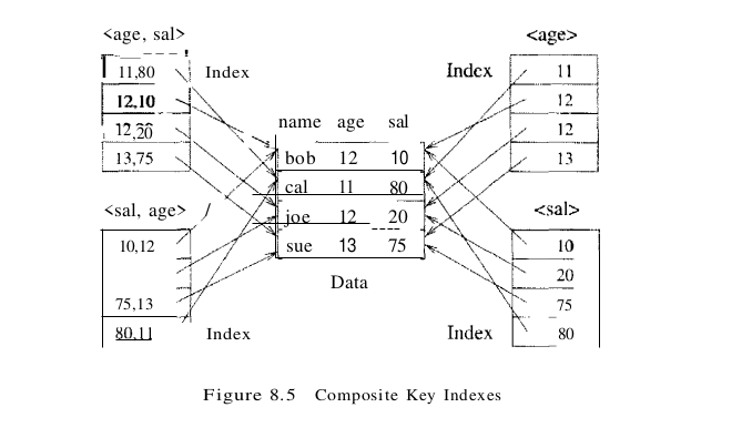
If the search key is composite, an equality query is one in which each field in the search key is bound to a constant. For example, we can ask to retrieve all data entries with age = 20 and sal = 10. The hashed file organization supports only equality queries, since a hash function identifies the bucket containing desired records only if a value is specified for each field in the search key.
A composite key index can support a broader range of queries because it matches more selection conditions. Further, since data entries in a composite index contain more information about the data record (i.e., more fields than a single-attribute index), the opportunities for index-only evaluation strategies are increased. On the negative side, a composite index must be updated in response to any operation (insert, delete, or update) that modifies any field in the search key. A composite index is also likely to be larger than a single-attribute search key index because the size of entries is larger.