- Forwarding and Routing
- Virtual Circuit and Datagram Networks
- The Internet Protocol (IP): Forwarding and Addressing in the Internet
- Internet Control Message Protocol (ICMP)
- IPv6
- Routing Algorithm
- Autonomous Systems (ASs)
- Broadcast Routing
- Spanning-Tree Broadcast
- Multicast Routing
The network service model defines the characteristics of end-to-end transport of packets between sending and receiving end systems.

Forwarding and Routing
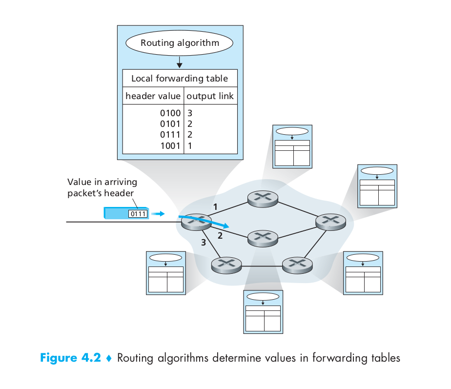
Forwarding involves the transfer of a packet from an incoming link to an outgoing link within a single router.
Every router has a forwarding table. A router forwards a packet by examining the value of a field in the arriving packet’s header, and then using this header value to index into the router’s forwarding table. The value stored in the forwarding table entry for that header indicates the router’s outgoing link interface to which that packet is to be forwarded. Depending on the network-layer protocol, the header value could be the destination address of the packet or an indication of the connection to which the packet belongs. And the routing algorithm determines the values that are inserted into the routers’ forwarding tables. The routing algorithm may be centralized or decentralized
Routing involves all of a network’s routers, whose collective interactions via routing protocols determine the paths that packets take on their trips from source to destination node.
Virtual Circuit and Datagram Networks
A network layer can provide connectionless service or connection service between two hosts. In all major computer network architectures to date (Internet, ATM, frame relay, and so on), the network layer provides either a host-to-host connectionless service or a host-to-host connection service, but not both. Computer networks that provide only a connection service at the network layer are called virtual-circuit (VC) networks; computer networks that provide only a connectionless service at the network layer are called datagram networks.
Internet is a datagram network while ATM and frame delay are VC networks.
The Internet Protocol (IP): Forwarding and Addressing in the Internet

- Version number. These 4 bits specify the IP protocol version of the datagram. By looking at the version number, the router can determine how to interpret the remainder of the IP datagram. Different versions of IP use different datagram formats.
- Header length. Because an IPv4 datagram can contain a variable number of options (which are included in the IPv4 datagram header), these 4 bits are needed to determine where in the IP datagram the data actually begins. Most IP datagrams do not contain options, so the typical IP datagram has a 20-byte header.
- Type of service. The type of service (TOS) bits were included in the IPv4 header to allow different types of IP datagrams (for example, datagrams particularly requiring low delay, high throughput, or reliability) to be distinguished from each other. For example, it might be useful to distinguish real-time datagrams (such as those used by an IP telephony application) from non-real-time traffic (for example, FTP). The specific level of service to be provided is a policy issue determined by the router’s administrator.
- Datagram length. This is the total length of the IP datagram (header plus data), measured in bytes. Since this field is 16 bits long, the theoretical maximum size of the IP datagram is 65,535 bytes. However, datagrams are rarely larger than 1,500 bytes.
- Identifier, flags, fragmentation offset. These three fields have to do with so-called IP fragmentation, a topic we will consider in depth shortly. Interestingly, the new version of IP, IPv6, does not allow for fragmentation at routers.
- Time-to-live. The time-to-live (TTL) field is included to ensure that datagrams do not circulate forever (due to, for example, a long-lived routing loop) in the network. This field is decremented by one each time the datagram is processed by a router. If the TTL field reaches 0, the datagram must be dropped.
- Protocol. This field is used only when an IP datagram reaches its final destination. The value of this field indicates the specific transport-layer protocol to which the data portion of this IP datagram should be passed. For example, a value of 6 indicates that the data portion is passed to TCP, while a value of 17 indicates that the data is passed to UDP. For a list of all possible values, see [IANA Protocol Numbers 2012]. Note that the protocol number in the IP datagram has a role that is analogous to the role of the port number field in the transport-layer segment. The protocol number is the glue that binds the network and transport layers together, whereas the port number is the glue that binds the transport and application layers together.
- Header checksum. The header checksum aids a router in detecting bit errors in a received IP datagram. The header checksum is computed by treating each 2 bytes in the header as a number and summing these numbers using 1s complement arithmetic. A router computes the header checksum for each received IP datagram and detects an error condition if the checksum carried in the datagram header does not equal the computed checksum. Routers typically discard datagrams for which an error has been detected. Note that the checksum must be recomputed and stored again at each router, as the TTL field, and possibly the options field as well, may change. An interesting discussion of fast algorithms for computing the Internet checksum is [RFC 1071]. A question often asked at this point is, why does TCP/IP perform error checking at both the transport and network layers? There are several reasons for this repetition. First, note that only the IP header is checksummed at the IP layer, while the TCP/UDP checksum is computed over the entire TCP/UDP segment. Second, TCP/UDP and IP do not necessarily both have to belong to the same protocol stack. TCP can, in principle, run over a different protocol (for example, ATM) and IP can carry data that will not be passed to TCP/UDP.
- Source and destination IP addresses. When a source creates a datagram, it inserts its IP address into the source IP address field and inserts the address of the ultimate destination into the destination IP address field. Often the source host determines the destination address via a DNS lookup.
- Options. The options fields allow an IP header to be extended. Header options were meant to be used rarely – hence the decision to save overhead by not including the information in options fields in every datagram header. However, the mere existence of options does complicate matters – since datagram headers can be of variable length, one cannot determine a priori where the data field will start. Also, since some datagrams may require options processing and others may not, the amount of time needed to process an IP datagram at a router can vary greatly. These considerations become particularly important for IP processing in high-performance routers and hosts. For these reasons and others, IP options were dropped in the IPv6 header.
- Data (payload). Finally, we come to the last and most important field – the raison d’être for the datagram in the first place! In most circumstances, the data field of the IP datagram contains the transport-layer segment (TCP or UDP) to be delivered to the destination. However, the data field can carry other types of data, such as ICMP messages.
IP Datagram Fragmentation
Imagine that you are a router that interconnects several links, each running different link-layer protocols with different MTUs. Suppose you receive an IP datagram from one link. You check your forwarding table to determine the outgoing link, and this outgoing link has an MTU that is smaller than the length of the IP datagram. Time to panic – how are you going to squeeze this oversized IP datagram into the payload field of the link-layer frame? The solution is to fragment the data in the IP datagram into two or more smaller IP datagrams, encapsulate each of these smaller IP datagrams in a separate link-layer frame; and send these frames over the outgoing link. Each of these smaller datagrams is referred to as a fragment.
Fragments need to be reassembled before they reach the transport layer at the destination. Sticking to the principle of keeping the network core simple, the designers of IPv4 decided to put the job of datagram reassembly in the end systems rather than in network routers. At the destination, the payload of the datagram is passed to the transport layer only after the IP layer has fully reconstructed the original IP datagram. If one or more of the fragments does not arrive at the destination, the incomplete datagram is discarded and not passed to the transport layer.
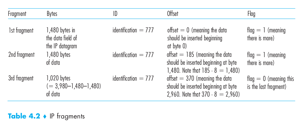
Suppose that a datagram of 4,000 bytes (20 bytes of IP header plus 3,980 bytes of IP payload) arrives at a router and must be forwarded to a link with an MTU of 1,500 bytes. This implies that the 3,980 data bytes in the original datagram must be allocated to three separate fragments (each of which is also an IP datagram). Suppose that the original datagram is stamped with an identification number of 777. The following image shows the fragments of this datagram.
IPv4 Addressing
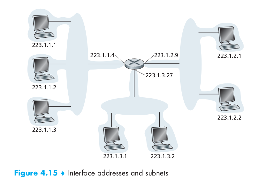
A host typically has only a single link into the network; when IP in the host wants to send a datagram, it does so over this link. The boundary between the host and the physical link is called an interface. The boundary between the router and any one of its links is also called an interface. A router thus has multiple interfaces, one for each of its links. Because every host and router is capable of sending and receiving IP datagrams, IP requires each host and router interface to have its own IP address. Thus, an IP address is technically associated with an interface, rather than with the host or router containing that interface. Each interface on every host and router in the global Internet must have an IP address that is globally unique (except for interfaces behind NATs).
In the following figure, one router (with three interfaces) is used to interconnect seven hosts. The three hosts in the upper-left portion of Figure 4.15, and the router interface to which they are connected, all have an IP address of the form 223.1.1.xxx. That is, they all have the same leftmost 24 bits in their IP address. The four interfaces are also interconnected to each other by a network that contains no routers. This network could be interconnected by an Ethernet LAN, in which case the interfaces would be interconnected by an Ethernet switch, or by a wireless access point. In IP terms, this network interconnecting three host interfaces and one router interface forms a subnet [RFC 950]. (A subnet is also called an IP network or simply a network in the Internet literature.) IP addressing assigns an address to this subnet: 223.1.1.0/24, where the /24 notation, sometimes known as a subnet mask, indicates that the leftmost 24 bits of the 32-bit quantity define the subnet address. The subnet 223.1.1.0/24 thus consists of the three host interfaces (223.1.1.1, 223.1.1.2, and 223.1.1.3) and one router interface (223.1.1.4). Any additional hosts attached to the 223.1.1.0/24 subnet would be required to have an address of the form 223.1.1.xxx.
Classless Interdomain Routing (CIDR)
The Internet’s address assignment strategy is known as Classless Interdomain Routing (CIDR – pronounced cider) [RFC 4632]. CIDR generalizes the notion of subnet addressing. As with subnet addressing, the 32-bit IP address is divided into two parts and again has the dotted-decimal form a.b.c.d/x, where x indicates the number of bits in the first part of the address. The x most significant bits of an address of the form a.b.c.d/x constitute the network portion of the IP address, and are often referred to as the prefix (or network prefix) of the address. An organization is typically assigned a block of contiguous addresses, that is, a range of addresses with a common prefix. In this case, the IP addresses of devices within the organization will share the common prefix.
Dynamic Host Configuraton Protocol (DHCP)
DHCP[RFC 2131] allows a host to obtain (be allocated) an IP address automatically. A network administrator can configure DHCP so that a given host receives the same IP address each time it connects to the network, or a host may be assigned a temporary IP address that will be different each time the host connects to the network. In addition to host IP address assignment, DHCP also allows a host to learn additional information, such as its subnet mask, the address of its first-hop router (often called the default gateway), and the address of its local DNS server.
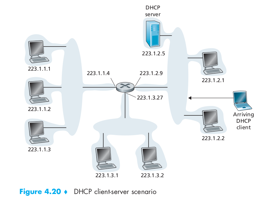
DHCP is a client-server protocol. A client is typically a newly arriving host wanting to obtain network configuration information, including an IP address for itself. In the simplest case, each subnet will have a DHCP server. If no server is present on the subnet, a DHCP relay agent (typically a router) that knows the address of a DHCP server for that network is needed. The following Figure 4.20 shows a DHCP server attached to subnet 223.1.2/24, with the router serving as the relay agent for arriving clients attached to subnets 223.1.1/24 and 223.1.3/24.
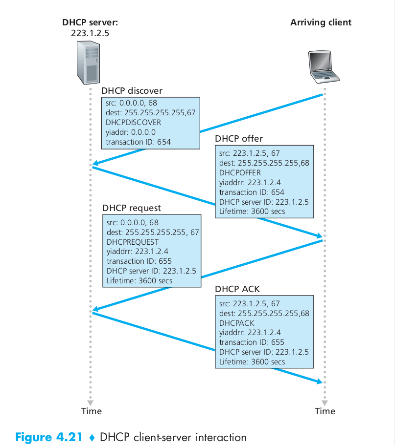
For a newly arriving host, the DHCP protocol is a four-step process, as shown in Figure 4.21 for the network setting shown in Figure 4.20. In this figure, yiaddr (as in “your Internet address”) indicates the address being allocated to the newly arriving client. The four steps are:
- DHCP server discovery. The first task of a newly arriving host is to find a DHCP server with which to interact. This is done using a DHCP discover message, which a client sends within a UDP packet to port 67. The UDP packet is encapsulated in an IP datagram. But to whom should this datagram be sent? The host doesn’t even know the IP address of the network to which it is attaching, much less the address of a DHCP server for this network. Given this, the DHCP client creates an IP datagram containing its DHCP discover message along with the broadcast destination IP address of 255.255.255.255 and a “this host” source IP address of 0.0.0.0. The DHCP client passes the IP datagram to the link layer, which then broadcasts this frame to all nodes attached to the subnet.
- DHCP server offer(s). A DHCP server receiving a DHCP discover message responds to the client with a DHCP offer message that is broadcast to all nodes on the subnet, again using the IP broadcast address of 255.255.255.255. (You might want to think about why this server reply must also be broadcast). Since several DHCP servers can be present on the subnet, the client may find itself in the enviable position of being able to choose from among several offers. Each server offer message contains the transaction ID of the received discover message, the proposed IP address for the client, the network mask, and an IP address lease time – the amount of time for which the IP address will be valid. It is common for the server to set the lease time to several hours or days.
- DHCP request. The newly arriving client will choose from among one or more server offers and respond to its selected offer with a DHCP request message, echoing back the configuration parameters.
- DHCP ACK. The server responds to the DHCP request message with a DHCP ACK message, confirming the requested parameters.
Network Address Translation (NAT)
IP Network Address Translation (NAT) was originally developed to solve the problem of a limited number of Internet IPv4 addresses. The need for NAT arises when multiple devices need to access the Internet but only one IPv4 Internet address is assigned by the Internet Service Provider (ISP).

Consider the example in Figure 4.22. Suppose a user sitting in a home network behind host 10.0.0.1 requests a Web page on some Web server (port 80) with IP address 128.119.40.186. The host 10.0.0.1 assigns the (arbitrary) source port number 3345 and sends the datagram into the LAN. The NAT router receives the datagram, generates a new source port number 5001 for the datagram, replaces the source IP address with its WAN-side IP address 138.76.29.7, and replaces the original source port number 3345 with the new source port number 5001. When generating a new source port number, the NAT router can select any source port number that is not currently in the NAT translation table. (Note that because a port number field is 16 bits long, the NAT protocol can support over 60,000 simultaneous connections with a single WAN-side IP address for the router!) NAT in the router also adds an entry to its NAT translation table. The Web server, blissfully unaware that the arriving datagram containing the HTTP request has been manipulated by the NAT router, responds with a datagram whose destination address is the IP address of the NAT router, and whose destination port number is 5001. When this datagram arrives at the NAT router, the router indexes the NAT translation table using the destination IP address and destination port number to obtain the appropriate IP address (10.0.0.1) and destination port number (3345) for the browser in the home network. The router then rewrites the datagram’s destination address and destination port number, and forwards the datagram into the home network.
There are some problems with NAT. First, port numbers are meant to be used for addressing processes, not for addressing hosts. Second, routers are supposed to process packets only up to layer 3(network layer). Third, the NAT protocol violates the so-called end-to-end argument; that is, hosts should be talking directly with each other, without interfering nodes modifying IP addresses and port numbers. And fourth, we should use IPv6 to solve the shortage of IP addresses, rather than recklessly patching up the problem with a stopgap solution like NAT. But like it or not, NAT has become an important component of the Internet. Yet another major problem with NAT is that it interferes with P2P applications, including P2P file-sharing applications and P2P Voice-over-IP applications. In a P2P application, any participating Peer A should be able to initiate a TCP connection to any other participating Peer B. The essence of the problem is that if Peer B is behind a NAT, it cannot act as a server and accept TCP connections. This NAT problem can be circumvented if Peer A is not behind a NAT. In this case, Peer A can first contact Peer B through an intermediate Peer C, which is not behind a NAT and to which B has established an ongoing TCP connection. Peer A can then ask Peer B, via Peer C, to initiate a TCP connection directly back to Peer A. Once the direct P2P TCP connection is established between Peers A and B, the two peers can exchange messages or files. This hack, called connection reversal, is actually used by many P2P applications for NAT traversal. If both Peer A and Peer B are behind their own NATs, the situation is a bit trickier but can be handled using application relays. For more details about the P2P communication across the NAT, you can read this document about “hole punching”.
NAT traversal is increasingly provided by Universal Plug and Play (UPnP), which is a protocol that allows a host to discover and configure a nearby NAT. UPnP requires that both the host and the NAT be UPnP compatible. With UPnP, an application running in a host can request a NAT mapping between its (private IP address, private port number) and the (public IP address, public port number) for some requested public port number. If the NAT accepts the request and creates the mapping, then nodes from the outside can initiate TCP connections to (public IP address, public port number). Furthermore, UPnP lets the application know the value of (public IP address, public port number), so that the application can advertise it to the outside world. As an example, suppose your host, behind a UPnP-enabled NAT, has private address 10.0.0.1 and is running BitTorrent on port 3345. Also suppose that the public IP address of the NAT is 138.76.29.7. Your BitTorrent application naturally wants to be able to accept connections from other hosts, so that it can trade chunks with them. To this end, the BitTorrent application in your host asks the NAT to create a “hole” that maps (10.0.0.1, 3345) to (138.76.29.7, 5001). (The public port number 5001 is chosen by the application.) The BitTorrent application in your host could also advertise to its tracker that it is available at (138.76.29.7, 5001). In this manner, an external host running BitTorrent can contact the tracker and learn that your BitTorrent application is running at (138.76.29.7, 5001). The external host can send a TCP SYN packet to (138.76.29.7, 5001). When the NAT receives the SYN packet, it will change the destination IP address and port number in the packet to (10.0.0.1, 3345) and forward the packet through the NAT.
Internet Control Message Protocol (ICMP)
ICMP, specified in [RFC 792], is used by hosts and routers to communicate network-layer information to each other. The most typical use of ICMP is for error reporting.
ICMP is often considered part of IP but architecturally it lies just above IP, as ICMP messages are carried inside IP datagrams. That is, ICMP messages are carried as IP payload, just as TCP or UDP segments are carried as IP payload. Similarly, when a host receives an IP datagram with ICMP specified as the upper-layer protocol, it demultiplexes the datagram’s contents to ICMP, just as it would demultiplex a datagram’s content to TCP or UDP.

IPv6
The format of the IPv6 datagram is shown in Figure 4.24. The most important changes introduced in IPv6 are evident in the datagram format:

- Expanded addressing capabilities. IPv6 increases the size of the IP address from 32 to 128 bits. This ensures that the world won’t run out of IP addresses. Now, every grain of sand on the planet can be IP-addressable. In addition to unicast and multicast addresses, IPv6 has introduced a new type of address, called an anycast address, which allows a datagram to be delivered to any one of a group of hosts. (This feature could be used, for example, to send an HTTP GET to the nearest of a number of mirror sites that contain a given document.)
- A streamlined 40-byte header. As discussed below, a number of IPv4 fields have been dropped or made optional. The resulting 40-byte fixed-length header allows for faster processing of the IP datagram. A new encoding of options allows for more flexible options processing.
- Flow labeling and priority. IPv6 has an elusive definition of a flow. RFC 1752 and RFC 2460 state that this allows “labeling of packets belonging to particular flows for which the sender requests special handling, such as a nondefault quality of service or real-time service.” For example, audio and video transmission might likely be treated as a flow. On the other hand, the more traditional applications, such as file transfer and e-mail, might not be treated as flows. It is possible that the traffic carried by a high-priority user (for example, someone paying for better service for their traffic) might also be treated as a flow. What is clear, however, is that the designers of IPv6 foresee the eventual need to be able to differentiate among the flows, even if the exact meaning of a flow has not yet been determined. The IPv6 header also has an 8-bit traffic class field. This field, like the TOS field in IPv4, can be used to give priority to certain datagrams within a flow, or it can be used to give priority to datagrams from certain applications (for example, ICMP) over datagrams from other applications (for example, network news).
As noted above, a comparison of Figure 4.24 with Figure 4.13 reveals the simpler, more streamlined structure of the IPv6 datagram. The following fields are defined in IPv6:
- Version. This 4-bit field identifies the IP version number. Not surprisingly, IPv6 carries a value of 6 in this field. Note that putting a 4 in this field does not create a valid IPv4 datagram. (If it did, life would be a lot simpler – see the discussion below regarding the transition from IPv4 to IPv6.)
- Traffic class. This 8-bit field is similar in spirit to the TOS field we saw in IPv4.
- Flow label. As discussed above, this 20-bit field is used to identify a flow of datagrams.
- Payload length. This 16-bit value is treated as an unsigned integer giving the number of bytes in the IPv6 datagram following the fixed-length, 40-byte datagram header.
- Next header. This field identifies the protocol to which the contents (data field) of this datagram will be delivered (for example, to TCP or UDP). The field uses the same values as the protocol field in the IPv4 header.
- Hop limit. The contents of this field are decremented by one by each router that forwards the datagram. If the hop limit count reaches zero, the datagram is discarded.
- Source and destination addresses. The various formats of the IPv6 128-bit address are described in RFC 4291.
- Data. This is the payload portion of the IPv6 datagram. When the datagram reaches its destination, the payload will be removed from the IP datagram and passed on to the protocol specified in the next header field.
The discussion above identified the purpose of the fields that are included in the IPv6 datagram. Comparing the IPv6 datagram format in Figure 4.24 with the IPv4 datagram format that we saw in Figure 4.13, we notice that several fields appearing in the IPv4 datagram are no longer present in the IPv6 datagram:
- Fragmentation/Reassembly. IPv6 does not allow for fragmentation and reassembly at intermediate routers; these operations can be performed only by the source and destination. If an IPv6 datagram received by a router is too large to be forwarded over the outgoing link, the router simply drops the datagram and sends a “Packet Too Big” ICMPv6 error message back to the sender. The sender can then resend the data, using a smaller IP datagram size. Fragmentation and reassembly is a time-consuming operation; removing this functionality from the routers and placing it squarely in the end systems considerably speeds up IP forwarding within the network.
- Header checksum. Because the transport-layer (for example, TCP and UDP) and link-layer (for example, Ethernet) protocols in the Internet layers perform checksumming, the designers of IP probably felt that this functionality was sufficiently redundant in the network layer that it could be removed. Once again, fast processing of IP packets was a central concern. Since the IPv4 header contains a TTL field (similar to the hop limit field in IPv6), the IPv4 header checksum needed to be recomputed at every router. As with fragmentation and reassembly, this too was a costly operation in IPv4.
- Options. An options field is no longer a part of the standard IP header. However, it has not gone away. Instead, the options field is one of the possible next headers pointed to from within the IPv6 header. That is, just as TCP or UDP protocol headers can be the next header within an IP packet, so too can an options field. The removal of the options field results in a fixed-length, 40-byte IP header.
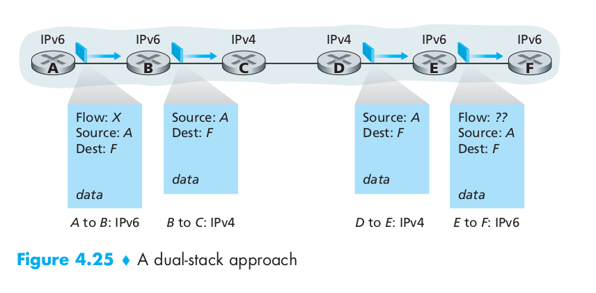
For the transition from IPv4 to IPv6, the most straightforward way to introduce IPv6-capable nodes is a dual-stack approach, where IPv6 nodes also have a complete IPv4 implementation. Such a node, referred to as an IPv6/IPv4 node in RFC 4213, has the ability to send and receive both IPv4 and IPv6 datagrams.
In the dual-stack approach, if either the sender or the receiver is only IPv4-capable, an IPv4 datagram must be used. As a result, it is possible that two IPv6-capable nodes can end up, in essence, sending IPv4 datagrams to each other. This is illustrated in Figure 4.25. Suppose Node A is IPv6-capable and wants to send an IP datagram to Node F, which is also IPv6-capable. Nodes A and B can exchange an IPv6 datagram. However, Node B must create an IPv4 datagram to send to C. Certainly, the data field of the IPv6 datagram can be copied into the data field of the IPv4 datagram and appropriate address mapping can be done. However, in performing the conversion from IPv6 to IPv4, there will be IPv6-specific fields in the IPv6 datagram (for example, the flow identifier field) that have no counterpart in IPv4. The information in these fields will be lost. Thus, even though E and F can exchange IPv6 datagrams, the arriving IPv4 datagrams at E from D do not contain all of the fields that were in the original IPv6 datagram sent from A.
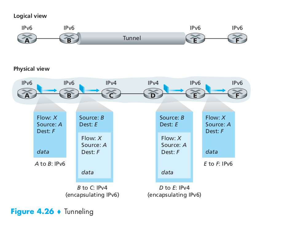
An alternative to the dual-stack approach, also discussed in RFC 4213, is known as tunneling. Tunneling can solve the problem noted above, allowing, for example, E to receive the IPv6 datagram originated by A. The basic idea behind tunneling is the following. Suppose two IPv6 nodes (for example, B and E in Figure 4.25) want to interoperate using IPv6 datagrams but are connected to each other by intervening IPv4 routers. We refer to the intervening set of IPv4 routers between two IPv6 routers as a tunnel, as illustrated in Figure 4.26. With tunneling, the IPv6 node on the sending side of the tunnel (for example, B) takes the entire IPv6 datagram and puts it in the data (payload) field of an IPv4 datagram. This IPv4 datagram is then addressed to the IPv6 node on the receiving side of the tunnel (for example, E) and sent to the first node in the tunnel (for example, C). The intervening IPv4 routers in the tunnel route this IPv4 datagram among themselves, just as they were any other datagram, blissfully unaware that the IPv4 datagram itself contains a complete IPv6 datagram. The IPv6 node on the receiving side of the tunnel eventually receives the IPv4 datagram (it is the destination of the IPv4 datagram!), determines that the IPv4 datagram contains an IPv6 datagram, extracts the IPv6 datagram, and then routes the IPv6 datagram exactly as it would if it had received the IPv6 datagram from a directly connected IPv6 neighbor.
Routing Algorithm
Typically a host is attached directly to one router, the default router for the host (also called the first-hop router for the host). Whenever a host sends a packet, the packet is transferred to its default router. We refer to the default router of the source host as the source router and the default router of the destination host as the destination router.
A global routing algorithm computes the least-cost path between a source and destination using complete, global knowledge about the network. That is, the algorithm takes the connectivity between all nodes and all link costs as inputs. This then requires that the algorithm somehow obtain this information before actually performing the calculation. The calculation itself can be run at one site (a centralized global routing algorithm) or replicated at multiple sites. The key distinguishing feature here, however, is that a global algorithm has complete information about connectivity and link costs. In practice, algorithms with global state information are often referred to as link-state (LS) algorithms, since the algorithm must be aware of the cost of each link in the network.
In a decentralized routing algorithm, the calculation of the least-cost path is carried out in an iterative, distributed manner. No node has complete information about the costs of all network links. Instead, each node begins with only the knowledge of the costs of its own directly attached links. Then, through an iterative process of calculation and exchange of information with its neighboring nodes (that is, nodes that are at the other end of links to which it itself is attached), a node gradually calculates the least-cost path to a destination or set of destinations. The decentralized routing algorithm we’ll study later is called a distance-vector (DV) algorithm, because each node maintains a vector of estimates of the costs (distances) to all other nodes in the network.
Link-State (LS) Routing Algorithm
In a link-state algorithm, the network topology and all link costs are known, that is, available as input to the LS algorithm. In practice this is accomplished by having each node broadcast link-state packets to all other nodes in the network, with each link-state packet containing the identities and costs of its attached links. In practice (for example, with the Internet’s OSPF routing protocol) this is often accomplished by a link-state broadcast algorithm. The result of the nodes’ broadcast is that all nodes have an identical and complete view of the network. Each node can then run the LS algorithm and compute the same set of least-cost paths as every other node.
The link-state routing algorithm we present below is known as Dijkstra’s algorithm. A closely related algorithm is Prim’s algorithm.
Let us define the following notation:
- D(v): cost of the least-cost path from the source node to destination v as of this iteration of the algorithm.
- p(v): previous node (neighbor of v) along the current least-cost path from the source to v.
- N’ : subset of nodes; v is in N’ if the least-cost path from the source to v is definitively known.


Distance Vector (DV) Routing Algorithm
Whereas the LS algorithm is an algorithm using global information, the distance-vector (DV) algorithm is iterative, asynchronous, and distributed. It is distributed in that each node receives some information from one or more of its directly attached neighbors, performs a calculation, and then distributes the results of its calculation back to its neighbors. It is iterative in that this process continues on until no more information is exchanged between neighbors. (Interestingly, the algorithm is also self-terminating – there is no signal that the computation should stop; it just stops.) The algorithm is asynchronous in that it does not require all of the nodes to operate in lockstep with each other.
Let $d_x(y)$ be the cost of the least-cost path from node x to node y. Then the least costs are related by the celebrated Bellman-Ford equation, namely,
\[d_{x}(y)=\min_{v}\left\{c(x, v)+d_{v}(y)\right\}\]where the $min_v$ in the equation is taken over all of x’s neighbors. Indeed, after traveling from x to v, if we then take the least-cost path from v to y, the path cost will be $c(x,v) + d_v(y)$. Since we must begin by traveling to some neighbor v, the least cost from x to y is the minimum of $c(x,v) + d_v(y)$ taken over all neighbors v.
In the distributed, asynchronous algorithm, from time to time, each node sends a copy of its distance vector to each of its neighbors. When a node x receives a new distance vector from any of its neighbors v, it saves v’s distance vector, and then uses the Bellman-Ford equation to update its own distance vector.
DV-like algorithms are used in many routing protocols in practice, including the Internet’s RIP and BGP, ISO IDRP, Novell IPX, and the original ARPAnet.
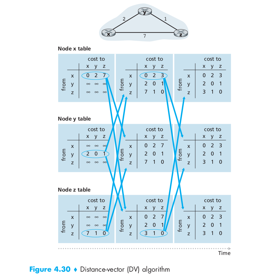
The following image shows a simple example of the distance vector algorithm.
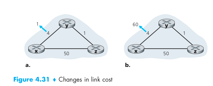
When a node running the DV algorithm detects a change in the link cost from itself to a neighbor, it updates its distance vector and, if there’s a change in the cost of the least-cost path, informs its neighbors of its new distance vector. Figure 4.31(a) illustrates a scenario where the link cost from y to x changes from 4 to 1. We focus here only on y’ and z’s distance table entries to destination x. The DV algorithm causes the following sequence of events to occur:
- At time $t_0$, y detects the link-cost change (the cost has changed from 4 to 1), updates its distance vector, and informs its neighbors of this change since its distance vector has changed.
- At time $t_1$, z receives the update from y and updates its table. It computes a new least cost to x (it has decreased from a cost of 5 to a cost of 2) and sends its new distance vector to its neighbors.
- At time $t_2$, y receives z’s update and updates its distance table. y’s least costs do not change and hence y does not send any message to z. The algorithm comes to a quiescent state.
If the link cost decreases as the Figure 4.31(a) shows, we can find that the decreased cost between x and y has propagated quickly through the network.
Let’s now consider what can happen when a link cost increases. Suppose that the link cost between x and y increases from 4 to 60, as shown in Figure 4.31(b). Before the link cost changes, $D_y (x) = 4, D_y (z) = 1, D_z (y) = 1, \text{and} D_z (x) = 5$. At time $t_0$ , y detects the link-cost change (the cost has changed from 4 to 60). y computes its new minimum-cost path to x to have a cost of
\[D_{y}(x)=\min \left\{c(y, x)+D_{x}(x), c(y, z)+D_{z}(x)\right\}=\min \{60+0,1+5\}=6\]Of course, with our global view of the network, we can see that this new cost via z is wrong. But the only information node y has is that its direct cost to x is 60 and that z has last told y that z could get to x with a cost of 5. So in order to get to x, y would now route through z, fully expecting that z will be able to get to x with a cost of 5. As of $t_1$ we have a routing loop – in order to get to x, y routes through z, and z routes through y. A routing loop is like a black hole – a packet destined for x arriving at y or z as of $t_1$ will bounce back and forth between these two nodes forever (or until the forwarding tables are changed). Sometime after $t_1$, z receives y’s new distance vector, which indicates that y’s minimum cost to x is 6. z knows it can get to y with a cost of 1 and hence computes a new least cost to x of $D_z(x)$ = min{50 + 0,1 + 6} = 7. Since z’s least cost to x has increased, it then informs y of its new distance vector at $t_2$. In a similar manner, after receiving z’s new distance vector, y determines $D_y(x)$ = 8 and sends z its distance vector. z then determines $D_z(x)$ = 9 and sends y its distance vector, and so on.
How long will the process continue? You should convince yourself that the loop will persist for 44 iterations (message exchanges between y and z) – until z eventually computes the cost of its path via y to be greater than 50. At this point, z will (finally!) determine that its least-cost path to x is via its direct connection to x. y will then route to x via z. The result of the bad news about the increase in link cost has indeed traveled slowly!
The specific looping scenario just described can be avoided using a technique known as poisoned reverse. The idea is simple – if z routes through y to get to destination x, then z will advertise to y that its distance to x is infinity, that is, z will advertise to y that $D_z(x)$ = $\infty$ (even though z knows $D_z(x)$ = 5 in truth). z will continue telling this little white lie to y as long as it routes to x via y. Since y believes that z has no path to x, y will never attempt to route to x via z, as long as z continues to route to x via y (and lies about doing so).
Let’s now see how poisoned reverse solves the particular looping problem we encountered before in Figure 4.31(b). As a result of the poisoned reverse, y’s distance table indicates $D_z(x)$ = $\infty$. When the cost of the (x, y) link changes from 4 to 60 at time $t_0$, y updates its table and continues to route directly to x, albeit at a higher cost of 60, and informs z of its new cost to x, that is, $D_y(x)$ = 60. After receiving the update at $t_1$, z immediately shifts its route to x to be via the direct (z, x) link at a cost of 50. Since this is a new least-cost path to x, and since the path no longer passes through y, z now informs y that $D_z(x)$ = 50 at $t_2$. After receiving the update from z, y updates its distance table with $D_y(x)$ = 51. Also, since z is now on y’s least-cost path to x, y poisons the reverse path from z to x by informing z at time $t_3$ that $D_y(x)$ = $\infty$ (even though y knows that $D_y(x)$ = 51 in truth).
Does poisoned reverse solve the general count-to-infinity problem? It does not. You should convince yourself that loops involving three or more nodes (rather than simply two immediately neighboring nodes) will not be detected by the poisoned reverse technique.
Autonomous Systems (ASs)
With each AS consisting of a group of routers that are typically under the same administrative control (e.g., operated by the same ISP or belonging to the same company network). Routers within the same AS all run the same routing algorithm (for example, an LS or DV algorithm) and have information about each other – exactly as was the case in our idealized model in the preceding section. The routing algorithm running within an autonomous system is called an intra-autonomous system routing protocol. It will be necessary, of course, to connect ASs to each other, and thus one or more of the routers in an AS will have the added task of being responsible for forwarding packets to destinations outside the AS; these routers are called gateway routers.
Obtaining reachability information from neighboring ASs and propagating the reachability information to all routers internal to the AS – are handled by the inter-AS routing protocol. Since the inter-AS routing protocol involves communication between two ASs, the two communicating ASs must run the same inter-AS routing protocol. In fact, in the Internet all ASs run the same inter-AS routing protocol, called BGP4.
Intra-AS Routing in the internet: RIP
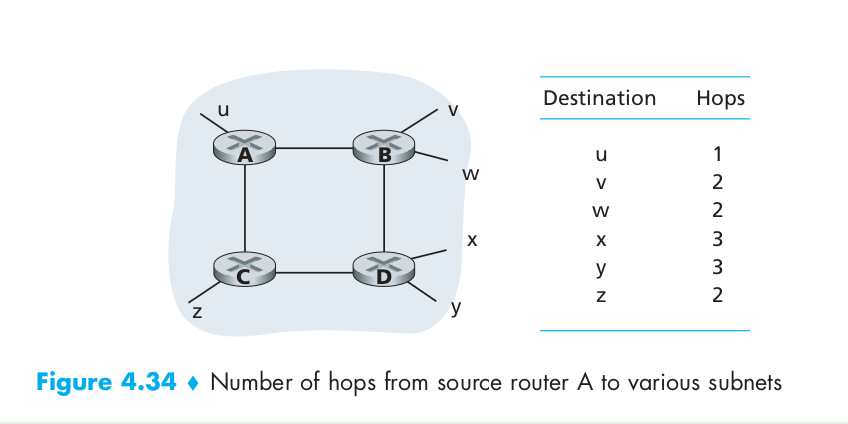
Routing Information Protocol (RIP) was one of the earliest intra-AS Internet routing protocols and is still in widespread use today. RIP is a distance-vector protocol that operates in a manner very close to the idealized DV protocol. The version of RIP specified in RFC 1058 uses hop count as a cost metric; that is, each link has a cost of 1. In RIP (and also in OSPF), costs are actually from source router to a destination subnet. RIP uses the term hop, which is the number of subnets traversed along the shortest path from source router to destination subnet, including the destination subnet. Figure 4.34 illustrates an AS with six leaf subnets. The table in the figure indicates the number of hops from the source A to each of the leaf subnets.
The maximum cost of a path is limited to 15, thus limiting the use of RIP to autonomous systems that are fewer than 15 hops in diameter. In RIP, routing updates are exchanged between neighbors approximately every 30 seconds using a RIP response message. The response message sent by a router or host contains a list of up to 25 destination subnets within the AS, as well as the sender’s distance to each of those subnets. Response messages are also known as RIP advertisements.
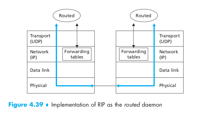
A router can also request information about its neighbor’s cost to a given destination using RIP’s request message. Routers send RIP request and response messages to each other over UDP using port number 520. The UDP segment is carried between routers in a standard IP datagram. Figure 4.39 sketches how RIP is typically implemented in a UNIX system, for example, a UNIX workstation serving as a router. A process called routed (pronounced “route dee”) executes RIP, that is, maintains routing information and exchanges messages with routed processes running in neighboring routers. Because RIP is implemented as an application-layer process (albeit a very special one that is able to manipulate the routing tables within the UNIX kernel), it can send and receive messages over a standard socket and use a standard transport protocol. As shown, RIP is implemented as an application-layer protocol running over UDP.
Intra-AS Routing in the internet: OSPF
Open Shortest Path First (OSPF) routing is widely used for intra-AS routing in the Internet. A routing protocol closely related to OSPF is the Intermediate-System-to-Intermediate-System (IS-IS) protocol [RFC 1142, Perlman 1999] and they are typically deployed in upper-tier ISPs whereas RIP is deployed in lower-tier ISPs and enterprise networks.
OSPF was conceived as the successor to RIP and as such has a number of advanced features. At its heart, however, OSPF is a link-state protocol that uses flooding of link-state information and a Dijkstra least-cost path algorithm. OSPF does not mandate a policy for how link weights are set (that is the job of the network administrator), but instead provides the mechanisms (protocol) for determining least-cost path routing for the given set of link weights.
With OSPF, a router broadcasts routing information to all other routers in the autonomous system, not just to its neighboring routers. A router broadcasts link-state information whenever there is a change in a link’s state (for example, a change in cost or a change in up/down status). It also broadcasts a link’s state periodically (at least once every 30 minutes), even if the link’s state has not changed. RFC 2328 notes that “this periodic updating of link state advertisements adds robustness to the link state algorithm.”
Inter-AS Routing in the internet: BGP
The Border Gateway Protocol version 4, specified in RFC 4271 (see also [RFC 4274), is the de facto standard inter-AS routing protocol in today’s Internet. It is commonly referred to as BGP4 or simply as BGP. BGP allows each subnet to advertise its existence to the rest of the Internet. A subnet screams “I exist and I am here,” and BGP makes sure that all the ASs in the Internet know about the subnet and how to get there.
Broadcast Routing
In broadcast routing, the network layer provides a service of delivering a packet sent from a source node to all other nodes in the network. Broadcast protocols are used in practice at both the application and network layers.
Uncontroled Flooding
The most obvious technique for achieving broadcast is a flooding approach in which the source node sends a copy of the packet to all of its neighbors. When a node receives a broadcast packet, it duplicates the packet and forwards it to all of its neighbors (except the neighbor from which it received the packet). Although this scheme is simple and elegant, it has a fatal flaw. If the graph has cycles, then one or more copies of each broadcast packet will cycle indefinitely. But there can be an even more calamitous fatal flaw: When a node is connected to more than two other nodes, it will create and forward multiple copies of the broadcast packet, each of which will create multiple copies of itself (at other nodes with more than two neighbors), and so on. This broadcast storm, resulting from the endless multiplication of broadcast packets, would eventually result in so many broadcast packets being created that the network would be rendered useless.
Controled Flooding
In sequence-number-controlled flooding, a source node puts its address (or other unique identifier) as well as a broadcast sequence number into a broadcast packet, then sends the packet to all of its neighbors. Each node maintains a list of the source address and sequence number of each broadcast packet it has already received, duplicated, and forwarded. When a node receives a broadcast packet, it first checks whether the packet is in this list. If so, the packet is dropped; if not, the packet is duplicated and forwarded to all the node’s neighbors.
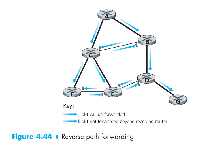
A second approach to controlled flooding is known as reverse path forwarding (RPF), also sometimes referred to as reverse path broadcast (RPB). RPF can avoid the broadcast storm. Figure 4.44 illustrates RPF. Suppose that the links drawn with thick lines represent the least-cost paths from the receivers to the source (A). Node A initially broadcasts a source-A packet to nodes C and B. Node B will forward the source-A packet it has received from A (since A is on its least-cost path to A) to both C and D. B will ignore (drop, without forwarding) any source-A packets it receives from any other nodes (for example, from routers C or D). Let us now consider node C, which will receive a source-A packet directly from A as well as from B. Since B is not on C’s own shortest path back to A, C will ignore any source-A packets it receives from B. On the other hand, when C receives a source-A packet directly from A, it will forward the packet to nodes B, E, and F.
Spanning-Tree Broadcast
While sequence-number-controlled flooding and RPF avoid broadcast storms, they do not completely avoid the transmission of redundant broadcast packets.
The main complexity associated with the spanning-tree approach is the creation and maintenance of the spanning tree. Numerous distributed spanning-tree algorithms have been developed. We consider only one simple algorithm here. In the center-based approach to building a spanning tree, a center node (also known as a rendezvous point or a core) is defined. Nodes then unicast tree-join messages addressed to the center node. A tree-join message is forwarded using unicast routing toward the center until it either arrives at a node that already belongs to the spanning tree or arrives at the center. In either case, the path that the tree-join message has followed defines the branch of the spanning tree between the edge node that initiated the tree-join message and the center. One can think of this new path as being grafted onto the existing spanning tree.
Figure 4.46 illustrates the construction of a center-based spanning tree. Suppose that node E is selected as the center of the tree. Suppose that node F first joins the tree and forwards a tree-join message to E. The single link EF becomes the initial spanning tree. Node B then joins the spanning tree by sending its tree-join message to E. Suppose that the unicast path route to E from B is via D. In this case, the tree-join message results in the path BDE being grafted onto the spanning tree. Node A next joins the spanning group by forwarding its tree-join message towards E. If A’s unicast path to E is through B, then since B has already joined the spanning tree, the arrival of A’s tree-join message at B will result in the AB link being immediately grafted onto the spanning tree. Node C joins the spanning tree next by forwarding its tree-join message directly to E. Finally, because the unicast routing from G to E must be via node D, when G sends its tree-join message to E, the GD link is grafted onto the spanning tree at node D.

Multicast Routing
multicast routing enables a single source node to send a copy of a packet to a subset of the other network nodes. In multicast communication, we are immediately faced with two problems – how to identify the receivers of a multicast packet and how to address a packet sent to these receivers. In the case of unicast communication, the IP address of the receiver (destination) is carried in each IP unicast datagram and identifies the single recipient; in the case of broadcast, all nodes need to receive the broadcast packet, so no destination addresses are needed.
In the Internet architecture (and other network architectures such as ATM), a multicast packet is addressed using address indirection. That is, a single identifier is used for the group of receivers, and a copy of the packet that is addressed to the group using this single identifier is delivered to all of the multicast receivers associated with that group. In the Internet, the single identifier that represents a group of receivers is a class D multicast IP address. The group of receivers associated with a class D address is referred to as a multicast group.
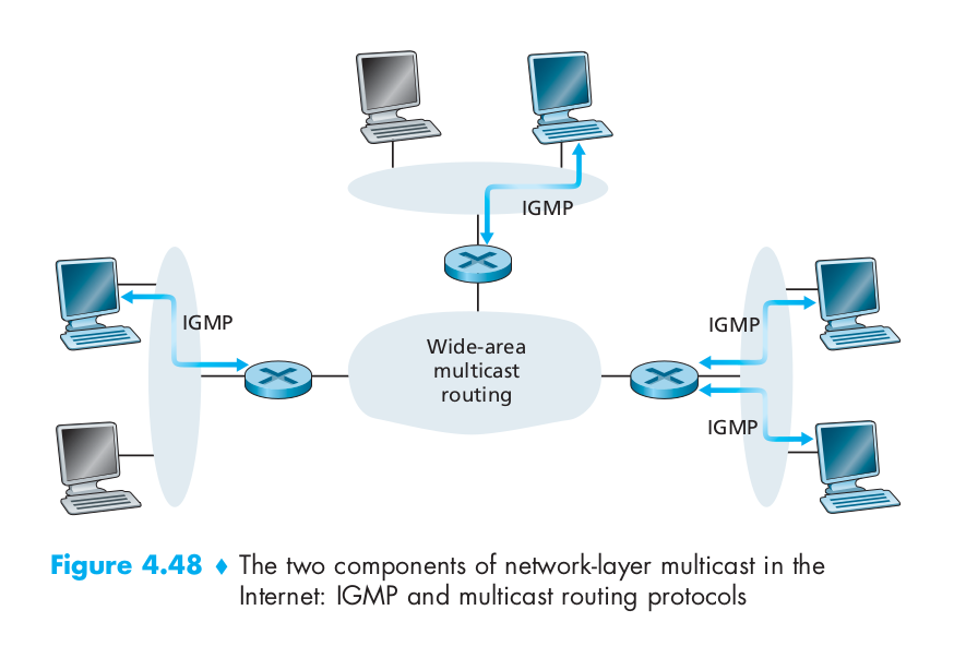
The Internet Group Management Protocol (IGMP) protocol version 3 [RFC 3376] operates between a host and its directly attached router (informally, we can think of the directly attached router as the first-hop router that a host would see on a path to any other host outside its own local network, or the last-hop router on any path to that host). IGMP provides the means for a host to inform its attached router that an application running on the host wants to join a specific multicast group. Given that the scope of IGMP interaction is limited to a host and its attached router, another protocol is clearly required to coordinate the multicast routers (including the attached routers) throughout the Internet, so that multicast datagrams are routed to their final destinations. This latter functionality is accomplished by network-layer multicast routing algorithms. Network-layer multicast in the Internet thus consists of two complementary components: IGMP and multicast routing protocols.
IGMP has only three message types. Like ICMP, IGMP messages are carried (encapsulated) within an IP datagram, with an IP protocol number of 2. The membership_query message is sent by a router to all hosts on an attached interface (for example, to all hosts on a local area network) to determine the set of all multicast groups that have been joined by the hosts on that interface. Hosts respond to a membership_query message with an IGMP membership_report message. membership_report messages can also be generated by a host when an application first joins a multicast group without waiting for a membership_query message from the router. The final type of IGMP message is the leave_group message. Interestingly, this message is optional. But if it is optional, how does a router detect when a host leaves the multicast group? The answer to this question is that the router infers that a host is no longer in the multicast group if it no longer responds to a membership_query message with the given group address. This is an example of what is sometimes called soft state in an Internet protocol. In a soft-state protocol, the state (in this case of IGMP, the fact that there are hosts joined to a given multicast group) is removed via a timeout event (in this case, via a periodic membership_query message from the router) if it is not explicitly refreshed (in this case, by a membership_report message from an attached host).
The goal of multicast routing, is to find a tree of links that connects all of the routers that have attached hosts belonging to the multicast group. Multicast packets will then be routed along this tree from the sender to all of the hosts belonging to the multicast tree. Of course, the tree may contain routers that do not have attached hosts belonging to the multicast group. In practice, two approaches have been adopted for determining the multicast routing tree. The two approaches differ according to whether a single group-shared tree is used to distribute the traffic for all senders in the group, or whether a source-specific routing tree is constructed for each individual sender.
- Multicast routing using a group-shared tree. As in the case of spanning-tree broadcast, multicast routing over a group-shared tree is based on building a tree that includes all edge routers with attached hosts belonging to the multicast group. In practice, a center-based approach is used to construct the multicast routing tree.
- Multicast routing using a source-based tree. While group-shared tree multicast routing constructs a single, shared routing tree to route packets from all senders, the second approach constructs a multicast routing tree for each source in the multicast group. In practice, an RPF algorithm (with source node x) is used to construct a multicast forwarding tree for multicast datagrams originating at source x. However, under broadcast RPF, it would forward packets to router even though the router has no attached hosts that are joined to the multicast group. The solution to the problem of receiving unwanted multicast packets under RPF is known as pruning. A multicast router that receives multicast packets and has no attached hosts joined to that group will send a prune message to its upstream router. If a router receives prune messages from each of its downstream routers, then it can forward a prune message upstream.
The first multicast routing protocol used in the Internet was the Distance-Vector Multicast Routing Protocol (DVMRP) [RFC 1075]. DVMRP implements source-based trees with reverse path forwarding and pruning. Perhaps the most widely used Internet multicast routing protocol is the Protocol-Independent Multicast (PIM) routing protocol, which explicitly recognizes two multicast distribution scenarios. In dense mode [RFC 3973], multicast group members are densely located; that is, many or most of the routers in the area need to be involved in routing multicast datagrams. PIM dense mode is a flood-and-prune reverse path forwarding technique similar in spirit to DVMRP. In sparse mode [RFC 4601], the number of routers with attached group members is small with respect to the total number of routers; group members are widely dispersed. PIM sparse mode uses rendezvous points to set up the multicast distribution tree. In source-specific multicast (SSM) [RFC 3569, RFC 4607], only a single sender is allowed to send traffic into the multicast tree, considerably simplifying tree construction and maintenance.