Multimedia Networking

• Multimedia Networking Applications
  • Properties of Video
  • Properties of Audio
  • Types of Multimedia Network Applications
• Streaming Stored Audio and Video
  • UDP Streaming
  • HTTP Streaming
    • Content Distribution Networks (CDNs)
• Conversational Voice-and Video-over-IP
• Streaming Live Audio and Video

Multimedia Networking Applications

Properties of Video

Perhaps the most salient characteristic of video is its high bit rate. Another important characteristic of video is that it can be compressed, thereby trading off video quality with bit rate. There are two types of redundancy in video, both of which can be exploited by video compression. Spatial redundancy is the redundancy within a given image. Intuitively, an image that consists of mostly white space has a high degree of redundancy and can be efficiently compressed without significantly sacrificing image quality. Temporal redundancy reflects repetition from image to subsequent image. If, for example, an image and the subsequent image are exactly the same, there is no reason to reencode the subsequent image; it is instead more efficient simply to indicate during encoding that the subsequent image is exactly the same.

Properties of Audio

Digital audio (including digitized speech and music) has significantly lower bandwidth requirements than video. Digital audio, however, has its own unique properties that must be considered when designing multimedia network applications. To understand these properties, let’s first consider how analog audio (which humans and musical instruments generate) is converted to a digital signal:

• The analog audio signal is sampled at some fixed rate, for example, at 8,000 samples per second. The value of each sample is an arbitrary real number.
• Each of the samples is then rounded to one of a finite number of values. This operation is referred to as quantization. The number of such finite values – called quantization values – is typically a power of two, for example, 256 quantization values.
• Each of the quantization values is represented by a fixed number of bits. For example, if there are 256 quantization values, then each value – and hence each audio sample – is represented by one byte. The bit representations of all the samples are then concatenated together to form the digital representation of the signal. As an example, if an analog audio signal is sampled at 8,000 samples per second and each sample is quantized and represented by 8 bits, then the resulting digital signal will have a rate of 64,000 bits per second. For playback through audio speakers, the digital signal can then be converted back – that is, decoded – to an analog signal. However, the decoded analog signal is only an approximation of the original signal, and the sound quality may be noticeably degraded (for example, high-frequency sounds may be missing in the decoded signal). By increasing the sampling rate and the number of quantization values, the decoded signal can better approximate the original analog signal. Thus (as with video), there is a trade-off between the quality of the decoded signal and the bit-rate and storage requirements of the digital signal.

The basic encoding technique that we just described is called pulse code modulation (PCM). Speech encoding often uses PCM, with a sampling rate of 8,000 samples per second and 8 bits per sample, resulting in a rate of 64 kbps. The audio compact disk (CD) also uses PCM, with a sampling rate of 44,100 samples per second with 16 bits per sample; this gives a rate of 705.6 kbps for mono and 1.411 Mbps for stereo. PCM-encoded speech and music, however, are rarely used in the Internet. Instead, as with video, compression techniques are used to reduce the bit rates of the stream. Human speech can be compressed to less than 10 kbps and still be intelligible. A popular compression technique for near CD-quality stereo music is MPEG Player 3, more commonly known as MP3. MP3 encoders can compress to many different rates; 128 kbps is the most common encoding rate and produces very little sound degradation. A related standard is Advanced Audio Coding (AAC), which has been popularized by Apple. As with video, multiple versions of a prerecorded audio stream can be created, each at a different bit rate.

Types of Multimedia Network Applications

The Internet supports a large variety of useful and entertaining multimedia applications. In this subsection, we classify multimedia applications into three broad categories: (i) streaming stored audio/video, (ii) conversational voice/video-over-IP, and (iii) streaming live audio/video. As we will soon see, each of these application categories has its own set of service requirements and design issues.

Streaming Stored Audio and Video

To keep the discussion concrete, we focus here on streaming stored video, which typically combines video and audio components. Streaming stored audio (such as streaming music) is very similar to streaming stored video, although the bit rates are typically much lower. In this class of applications, the underlying medium is prerecorded video, such as a movie, a television show, a prerecorded sporting event, or a prerecorded user-generated video (such as those commonly seen on YouTube). These prerecorded videos are placed on servers, and users send requests to the servers to view the videos on demand. Many Internet companies today provide streaming video, including YouTube (Google), Netflix, and Hulu. By some estimates, streaming stored video makes up over 50 percent of the downstream traffic in the Internet access networks today [Cisco 2011]. Streaming stored video has three key distinguishing features.

• Streaming. In a streaming stored video application, the client typically begins video playout within a few seconds after it begins receiving the video from the server. This means that the client will be playing out from one location in the video while at the same time receiving later parts of the video from the server. This technique, known as streaming, avoids having to download the entire video file (and incurring a potentially long delay) before playout begins.
• Interactivity. Because the media is prerecorded, the user may pause, reposition forward, reposition backward, fast-forward, and so on through the video content. The time from when the user makes such a request until the action manifests itself at the client should be less than a few seconds for acceptable responsiveness.
• Continuous playout. Once playout of the video begins, it should proceed according to the original timing of the recording. Therefore, data must be received from the server in time for its playout at the client; otherwise, users experience video frame freezing (when the client waits for the delayed frames) or frame skipping (when the client skips over delayed frames).

By far, the most important performance measure for streaming video is average throughput. In order to provide continuous playout, the network must provide an average throughput to the streaming application that is at least as large the bit rate of the video itself. By using buffering and prefetching, it is possible to provide continuous playout even when the throughput fluctuates, as long as the average throughput (averaged over 5–10 seconds) remains above the video rate.

Streaming video systems can be classified into three categories: UDP streaming, HTTP streaming, and adaptive HTTP streaming. Although all three types of systems are used in practice, the majority of today’s systems employ HTTP streaming and adaptive HTTP streaming. A common characteristic of all three forms of video streaming is the extensive use of client-side application buffering to mitigate the effects of varying end-to-end delays and varying amounts of available bandwidth between server and client. For streaming video (both stored and live), users generally can tolerate a small several-second initial delay between when the client requests a video and when video playout begins at the client. Consequently, when the video starts to arrive at the client, the client need not immediately begin playout, but can instead build up a reserve of video in an application buffer. Once the client has built up a reserve of several seconds of buffered-but-not-yet-played video, the client can then begin video playout. There are two important advantages provided by such client buffering. First, client-side buffering can absorb variations in server-to-client delay. If a particular piece of video data is delayed, as long as it arrives before the reserve of received-but-not-yet-played video is exhausted, this long delay will not be noticed. Second, if the server-to-client bandwidth briefly drops below the video consumption rate, a user can continue to enjoy continuous playback, again as long as the client application buffer does not become completely drained.

UDP Streaming

Before passing the video chunks to UDP, the server will encapsulate the video chunks within transport packets specially designed for transporting audio and video, using the Real-Time Transport Protocol (RTP) [RFC 3550] or a similar (possibly proprietary) scheme. Another distinguishing property of UDP streaming is that in addition to the server-to-client video stream, the client and server also maintain, in parallel, a separate control connection over which the client sends commands regarding session state changes (such as pause, resume, reposition, and so on). This control connection is in many ways analogous to the FTP control connection. The Real-Time Streaming Protocol (RTSP) [RFC 2326], explained in some detail in the companion Web site for this textbook, is a popular open protocol for such a control connection. Although UDP streaming has been employed in many open-source systems and proprietary products, it suffers from three significant drawbacks.

First, due to the unpredictable and varying amount of available bandwidth between server and client, constant-rate UDP streaming can fail to provide continuous playout. For example, consider the scenario where the video consumption rate is 1 Mbps and the server-to-client available bandwidth is usually more than 1 Mbps, but every few minutes the available bandwidth drops below 1 Mbps for several seconds. In such a scenario, a UDP streaming system that transmits video at a constant rate of 1 Mbps over RTP/UDP would likely provide a poor user experience, with freezing or skipped frames soon after the available bandwidth falls below 1 Mbps. The second drawback of UDP streaming is that it requires a media control server, such as an RTSP server, to process client-to-server interactivity requests and to track client state (e.g., the client’s playout point in the video, whether the video is being paused or played, and so on) for each ongoing client session. This increases the overall cost and complexity of deploying a large-scale video-on-demand system. The third drawback is that many firewalls are configured to block UDP traffic, preventing the users behind these firewalls from receiving UDP video.

HTTP Streaming

In HTTP streaming, the video is simply stored in an HTTP server as an ordinary file with a specific URL. When a user wants to see the video, the client establishes a TCP connection with the server and issues an HTTP GET request for that URL. The server then sends the video file, within an HTTP response message, as quickly as possible, that is, as quickly as TCP congestion control and flow control will allow. On the client side, the bytes are collected in a client application buffer. Once the number of bytes in this buffer exceeds a predetermined threshold, the client application begins playback – specifically, it periodically grabs video frames from the client application buffer, decompresses the frames, and displays them on the user’s screen. We learned that when transferring a file over TCP, the server-to-client transmission rate can vary significantly due to TCP’s congestion control mechanism. In particular, it is not uncommon for the transmission rate to vary in a “saw-tooth” manner associated with TCP congestion control. Furthermore, packets can also be significantly delayed due to TCP’s retransmission mechanism. Because of these characteristics of TCP, the conventional wisdom in the 1990s was that video streaming would never work well over TCP. Over time, however, designers of streaming video systems learned that TCP’s congestion control and reliable-data transfer mechanisms do not necessarily preclude continuous playout when client buffering and prefetching are used.

Although HTTP streaming has been extensively deployed in practice (for example, by YouTube since its inception), it has a major shortcoming: All clients receive the same encoding of the video, despite the large variations in the amount of bandwidth available to a client, both across different clients and also over time for the same client. This has led to the development of a new type of HTTP-based streaming, often referred to as Dynamic Adaptive Streaming over HTTP (DASH). In DASH, the video is encoded into several different versions, with each version having a different bit rate and, correspondingly, a different quality level. The client dynamically requests chunks of video segments of a few seconds in length from the different versions. When the amount of available bandwidth is high, the client naturally selects chunks from a high-rate version; and when the available bandwidth is low, it naturally selects from a low-rate version. The client selects different chunks one at a time with HTTP GET request messages. By dynamically monitoring the available bandwidth and client buffer level, and adjusting the transmission rate with version switching, DASH can often achieve continuous playout at the best possible quality level without frame freezing or skipping. Furthermore, since the client (rather than the server) maintains the intelligence to determine which chunk to send next, the scheme also improves server-side scalability. Another benefit of this approach is that the client can use the HTTP byte-range request to precisely control the amount of prefetched video that it buffers locally.

Content Distribution Networks (CDNs)

For an Internet video company, perhaps the most straightforward approach to providing streaming video service is to build a single massive data center, store all of its videos in the data center, and stream the videos directly from the data center to clients worldwide. But there are three major problems with this approach. First, if the client is far from the data center, server-to-client packets will cross many communication links and likely pass through many ISPs, with some of the ISPs possibly located on different continents. If one of these links provides a throughput that is less than the video consumption rate, the end-to-end throughput will also be below the consumption rate, resulting in annoying freezing delays for the user. A second drawback is that a popular video will likely be sent many times over the same communication links. Not only does this waste network bandwidth, but the Internet video company itself will be paying its provider ISP (connected to the data center) for sending the same bytes into the Internet over and over again. A third problem with this solution is that a single data center represents a single point of failure – if the data center or its links to the Internet goes down, it would not be able to distribute any video streams.

In order to meet the challenge of distributing massive amounts of video data to users distributed around the world, almost all major video-streaming companies make use of Content Distribution Networks (CDNs). A CDN manages servers in multiple geographically distributed locations, stores copies of the videos (and other types of Web content, including documents, images, and audio) in its servers, and attempts to direct each user request to a CDN location that will provide the best user experience. The CDN may be a private CDN, that is, owned by the content provider itself; for example, Google’s CDN distributes YouTube videos and other types of content. The CDN may alternatively be a third-party CDN that distributes content on behalf of multiple content providers; Akamai’s CDN, for example, is a third-party CDN that distributes Netflix and Hulu content, among others.

CDNs typically adopt one of two different server placement philosophies

• Enter Deep. One philosophy, pioneered by Akamai, is to enter deep into the access networks of Internet Service Providers, by deploying server clusters in access ISPs all over the world. Akamai takes this approach with clusters in approximately 1,700 locations. The goal is to get close to end users, thereby improving user-perceived delay and throughput by decreasing the number of links and routers between the end user and the CDN cluster from which it receives content. Because of this highly distributed design, the task of maintaining and managing the clusters becomes challenging.
• Bring Home. A second design philosophy, taken by Limelight and many other CDN companies, is to bring the ISPs home by building large clusters at a smaller number (for example, tens) of key locations and connecting these clusters using a private high-speed network. Instead of getting inside the access ISPs, these CDNs typically place each cluster at a location that is simultaneously near the PoPs of many tier-1 ISPs, for example, within a few miles of both AT&T and Verizon PoPs in a major city. Compared with the enter-deep design philosophy, the bring-home design typically results in lower maintenance and management overhead, possibly at the expense of higher delay and lower throughput to end users.

When a browser in a user’s host is instructed to retrieve a specific video (identified by a URL), the CDN must intercept the request so that it can (1) determine a suitable CDN server cluster for that client at that time, and (2) redirect the client’s request to a server in that cluster. Suppose a content provider, NetCinema, employs the third-party CDN company, KingCDN, to distribute its videos to its customers. On the NetCinema Web pages, each of its videos is assigned a URL that includes the string “video” and a unique identifier for the video itself; for example, Transformers 7 might be assigned http://video.netcinema.com/6Y7B23V. Six steps then occur, as shown in Figure 7.4:

1. The user visits the Web page at NetCinema.
2. When the user clicks on the link http://video.netcinema.com/6Y7B23V, the user’s host sends a DNS query for video.netcinema.com.
3. The user’s Local DNS Server (LDNS) relays the DNS query to an authoritative DNS server for NetCinema, which observes the string “video” in the hostname video.netcinema.com. To “hand over” the DNS query to KingCDN, instead of returning an IP address, the NetCinema authoritative DNS server returns to the LDNS a hostname in the KingCDN’s domain, for example, a1105.kingcdn.com.
4. From this point on, the DNS query enters into KingCDN’s private DNS infrastructure. The user’s LDNS then sends a second query, now for a1105.kingcdn.com, and KingCDN’s DNS system eventually returns the IP addresses of a KingCDN content server to the LDNS. It is thus here, within the KingCDN’s DNS system, that the CDN server from which the client will receive its content is specified.
5. The LDNS forwards the IP address of the content-serving CDN node to the user’s host.
6. Once the client receives the IP address for a KingCDN content server, it establishes a direct TCP connection with the server at that IP address and issues an HTTP GET request for the video. If DASH is used, the server will first send to the client a manifest file with a list of URLs, one for each version of the video, and the client will dynamically select chunks from the different versions.

At the core of any CDN deployment is a cluster selection strategy, that is, a mechanism for dynamically directing clients to a server cluster or a data center within the CDN. As we just saw, the CDN learns the IP address of the client’s LDNS server via the client’s DNS lookup. After learning this IP address, the CDN needs to select an appropriate cluster based on this IP address. CDNs generally employ proprietary cluster selection strategies. We now briefly survey a number of natural approaches, each of which has its own advantages and disadvantages. One simple strategy is to assign the client to the cluster that is geographically closest. Using commercial geo-location databases (such as Quova [Quova 2012] and Max-Mind [MaxMind 2012]), each LDNS IP address is mapped to a geographic location. When a DNS request is received from a particular LDNS, the CDN chooses the geographically closest cluster, that is, the cluster that is the fewest kilometers from the LDNS “as the bird flies.” Such a solution can work reasonably well for a large fraction of the clients [Agarwal 2009]. However, for some clients, the solution may perform poorly, since the geographically closest cluster may not be the closest cluster along the network path. Furthermore, a problem inherent with all DNS-based approaches is that some end-users are configured to use remotely located LDNSs [Shaikh 2001; Mao 2002], in which case the LDNS location may be far from the client’s location. Moreover, this simple strategy ignores the variation in delay and available bandwidth over time of Internet paths, always assigning the same cluster to a particular client. In order to determine the best cluster for a client based on the current traffic conditions, CDNs can instead perform periodic real-time measurements of delay and loss performance between their clusters and clients. For instance, a CDN can have each of its clusters periodically send probes (for example, ping messages or DNS queries) to all of the LDNSs around the world. One drawback of this approach is that many LDNSs are configured to not respond to such probes. An alternative to sending extraneous traffic for measuring path properties is to use the characteristics of recent and ongoing traffic between the clients and CDN servers. For instance, the delay between a client and a cluster can be estimated by examining the gap between server-to-client SYNACK and client-to-server ACK during the TCP three-way handshake. Such solutions, however, require redirecting clients to (possibly) suboptimal clusters from time to time in order to measure the properties of paths to these clusters. Although only a small number of requests need to serve as probes, the selected clients can suffer significant performance degradation when receiving content (video or otherwise). Another alternative for cluster-to-client path probing is to use DNS query traffic to measure the delay between clients and clusters. Specifically, during the DNS phase (within Step 4 in Figure 7.4), the client’s LDNS can be occasionally directed to different DNS authoritative servers installed at the various cluster locations, yielding DNS traffic that can then be measured between the LDNS and these cluster locations. In this scheme, the DNS servers continue to return the optimal cluster for the client, so that delivery of videos and other Web objects does not suffer. A very different approach to matching clients with CDN servers is to use IP anycast [RFC 1546]. The idea behind IP anycast is to have the routers in the Internet route the client’s packets to the “closest” cluster, as determined by BGP. During the IP-anycast configuration stage, the CDN company assigns the same IP address to each of its clusters, and uses standard BGP to advertise this IP address from each of the different cluster locations. When a BGP router receives multiple route advertisements for this same IP address, it treats these advertisements as providing different paths to the same physical location (when, in fact, the advertisements are for different paths to different physical locations). Following standard operating procedures, the BGP router will then pick the “best” (for example, closest, as determined by AS-hop counts) route to the IP address according to its local route selection mechanism. For example, if one BGP route (corresponding to one location) is only one AS hop away from the router, and all other BGP routes (corresponding to other locations) are two or more AS hops away, then the BGP router would typically choose to route packets to the location that needs to traverse only one AS. After this initial configuration phase, the CDN can do its main job of distributing content. When any client wants to see any video, the CDN’s DNS returns the anycast address, no matter where the client is located. When the client sends a packet to that IP address, the packet is routed to the “closest” cluster as determined by the preconfigured forwarding tables, which were configured with BGP as just described. This approach has the advantage of finding the cluster that is closest to the client rather than the cluster that is closest to the client’s LDNS. However, the IP anycast strategy again does not take into account the dynamic nature of the Internet over short time scales.

Conversational Voice-and Video-over-IP

Real-time conversational voice over the Internet is often referred to as Internet telephony, since, from the user’s perspective, it is similar to the traditional circuit-switched telephone service. It is also commonly called Voice-over-IP (VoIP). Conversational video is similar, except that it includes the video of the participants as well as their voices.

Timing considerations and tolerance of data loss – are particularly important for conversational voice and video applications. Timing considerations are important because audio and video conversational applications are highly delay-sensitive. For a conversation with two or more interacting speakers, the delay from when a user speaks or moves until the action is manifested at the other end should be less than a few hundred milliseconds. For voice, delays smaller than 150 milliseconds are not perceived by a human listener, delays between 150 and 400 milliseconds can be acceptable, and delays exceeding 400 milliseconds can result in frustrating, if not completely unintelligible, voice conversations. On the other hand, conversational multimedia applications are loss-tolerant – occasional loss only causes occasional glitches in audio/video playback, and these losses can often be partially or fully concealed. These delay-sensitive but loss-tolerant characteristics are clearly different from those of elastic data applications such as Web browsing, e-mail, social networks, and remote login. For elastic applications, long delays are annoying but not particularly harmful; the completeness and integrity of the transferred data, however, are of paramount importance.

The Internet’s network-layer protocol, IP, provides best-effort service. That is to say the service makes its best effort to move each datagram from source to destinations quickly as possible but makes no promises whatsoever about getting the packet to the destination within some delay bound or about a limit on the percentage of packets lost. The lack of such guarantees poses significant challenges to the design of real-time conversational applications, which are acutely sensitive to packet delay, jitter, and loss.

Loss could be eliminated by sending the packets over TCP (which provides for reliable data transfer) rather than over UDP. However, retransmission mechanisms are often considered unacceptable for conversational real-time audio applications such as VoIP, because they increase end-to-end delay. Furthermore, due to TCP congestion control, packet loss may result in a reduction of the TCP sender’s transmission rate to a rate that is lower than the receiver’s drain rate, possibly leading to buffer starvation. This can have a severe impact on voice intelligibility at the receiver. For these reasons, most existing VoIP applications run over UDP by default. [Baset 2006] reports that UDP is used by Skype unless a user is behind a NAT or firewall that blocks UDP segments (in which case TCP is used). But losing packets is not necessarily as disastrous as one might think. Indeed, packet loss rates between 1 and 20 percent can be tolerated, depending on how voice is encoded and transmitted, and on how the loss is concealed at the receiver. For example, forward error correction (FEC) can help conceal packet loss. We’ll see below that with FEC, redundant information is transmitted along with the original information so that some of the lost original data can be recovered from the redundant information. Nevertheless, if one or more of the links between sender and receiver is severely congested, and packet loss exceeds 10 to 20 percent (for example, on a wireless link), then there is really nothing that can be done to achieve acceptable audio quality. Clearly, best-effort service has its limitations.

End-to-end delay is the accumulation of transmission, processing, and queuing delays in routers; propagation delays in links; and end-system processing delays. The receiving side of a VoIP application will typically disregard any packets that are delayed more than a certain threshold, for example, more than 400 msecs. Thus, packets that are delayed by more than the threshold are effectively lost. A crucial component of end-to-end delay is the varying queuing delays that a packet experiences in the network’s routers. Because of these varying delays, the time from when a packet is generated at the source until it is received at the receiver can fluctuate from packet to packet. This phenomenon is called jitter. If the receiver ignores the presence of jitter and plays out chunks as soon as they arrive, then the resulting audio quality can easily become unintelligible at the receiver. Fortunately, jitter can often be removed by using sequence numbers, timestamps, and a playout delay. For our VoIP application, where packets are being generated periodically, the receiver should attempt to provide periodic playout of voice chunks in the presence of random network jitter. This is typically done by combining the following two mechanisms:

• Prepending each chunk with a timestamp. The sender stamps each chunk with the time at which the chunk was generated.
• Delaying playout of chunks at the receiver. The playout delay of the received audio chunks must be long enough so that most of the packets are received before their scheduled playout times. This playout delay can either be fixed throughout the duration of the audio session or vary adaptively during the audio session lifetime.

We now briefly describe several schemes that attempt to preserve acceptable audio quality in the presence of packet loss. Such schemes are called loss recovery schemes. Here we define packet loss in a broad sense: A packet is lost either if it never arrives at the receiver or if it arrives after its scheduled playout time. VoIP applications often use some type of loss anticipation scheme. Two types of loss anticipation schemes are forward error correction (FEC) and interleaving. The basic idea of FEC is to add redundant information to the original packet stream. For the cost of marginally increasing the transmission rate, the redundant information can be used to reconstruct approximations or exact versions of some of the lost packets. we now outline two simple FEC mechanisms.

The first mechanism sends a redundant encoded chunk after every n chunks. The redundant chunk is obtained by exclusive OR-ing the n original chunks. In this manner if any one packet of the group of n + 1 packets is lost, the receiver can fully reconstruct the lost packet. But if two or more packets in a group are lost, the receiver cannot reconstruct the lost packets. By keeping n + 1, the group size, small, a large fraction of the lost packets can be recovered when loss is not excessive. However, the smaller the group size, the greater the relative increase of the transmission rate. In particular, the transmission rate increases by a factor of 1/n, so that, if n = 3, then the transmission rate increases by 33 percent. Furthermore, this simple scheme increases the playout delay, as the receiver must wait to receive the entire group of packets before it can begin playout. For more practical details about how FEC works for multimedia transport see [RFC 5109].

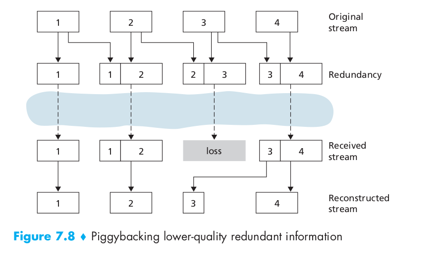
The second FEC mechanism is to send a lower-resolution audio stream as the redundant information. For example, the sender might create a nominal audio stream and a corresponding low-resolution, low-bit rate audio stream. (The nominal stream could be a PCM encoding at 64 kbps, and the lower-quality stream could be a GSM encoding at 13 kbps.) The low-bit rate stream is referred to as the redundant stream. As shown in Figure 7.8, the sender constructs the nth packet by taking the nth chunk from the nominal stream and appending to it the (n – 1)st chunk from the redundant stream. In this manner, whenever there is nonconsecutive packet loss, the receiver can conceal the loss by playing out the low-bit rate encoded chunk that arrives with the subsequent packet. In order to cope with consecutive loss, we can use a simple variation. Instead of appending just the (n – 1)st low-bit rate chunk to the nth nominal chunk, the sender can append the (n – 1)st and (n – 2)nd low-bit rate chunk, or append the (n – 1)st and (n – 3)rd low-bit rate chunk, and so on. By appending more low-bit rate chunks to each nominal chunk, the audio quality at the receiver becomes acceptable for a wider variety of harsh best-effort environments. On the other hand, the additional chunks increase the transmission bandwidth and the playout delay.

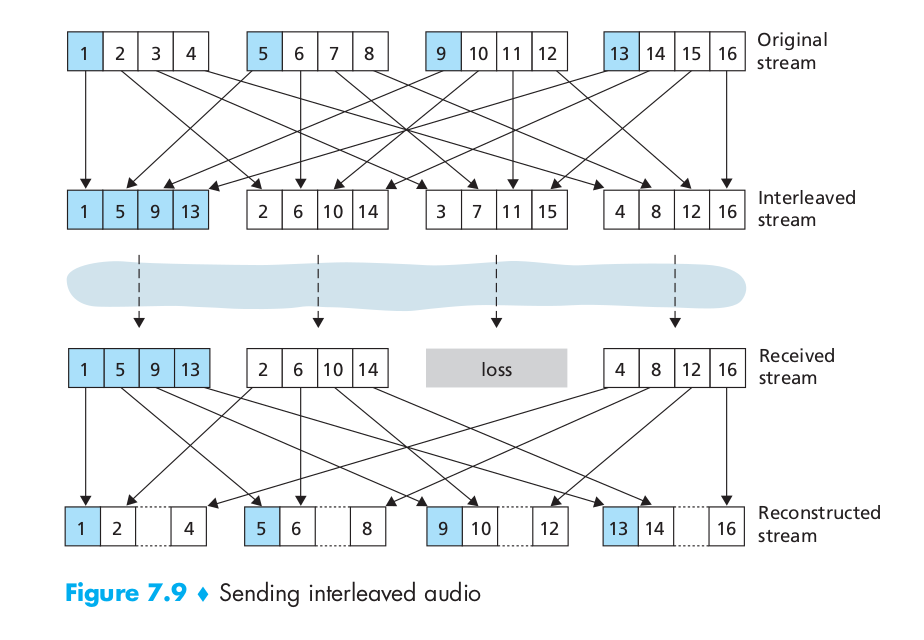
As an alternative to redundant transmission, a VoIP application can send interleaved audio. As shown in Figure 7.9, the sender resequences units of audio data before transmission, so that originally adjacent units are separated by a certain distance in the transmitted stream. Interleaving can mitigate the effect of packet losses. Interleaving can significantly improve the perceived quality of an audio stream. It also has low overhead. The obvious disadvantage of interleaving is that it increases latency. This limits its use for conversational applications such as VoIP, although it can perform well for streaming stored audio. A major advantage of interleaving is that it does not increase the bandwidth requirements of a stream.

Streaming Live Audio and Video

RTP,defined in RFC 3550, is such a standard. RTP can be used for transporting common formats such as PCM, ACC, and MP3 for sound and MPEG and H.263 for video. It can also be used for transporting proprietary sound and video formats. Today, RTP enjoys widespread implementation in many products and research prototypes. It is also complementary to other important real-time interactive protocols, such as SIP.

RTP typically runs on top of UDP. The sending side encapsulates a media chunk within an RTP packet, then encapsulates the packet in a UDP segment, and then hands the segment to IP. The receiving side extracts the RTP packet from the UDP segment, then extracts the media chunk from the RTP packet, and then passes the chunk to the media player for decoding and rendering. For example, image that the RTP is using to transport voice. The sending side precedes each chunk of the audio data with an RTP header that includes the type of audio encoding, a sequence number, and a timestamp. The RTP header is normally 12 bytes. The audio chunk along with the RTP header form the RTP packet. The RTP packet is then sent into the UDP socket interface. At the receiver side, the application receives the RTP packet from its socket interface. The application extracts the audio chunk from the RTP packet and uses the header fields of the RTP packet to properly decode and play back the audio chunk. If an application incorporates RTP – instead of a proprietary scheme to provide payload type, sequence numbers, or timestamps – then the application will more easily interoperate with other networked multimedia applications. For example, if two different companies develop VoIP software and they both incorporate RTP into their product, there may be some hope that a user using one of the VoIP products will be able to communicate with a user using the other VoIP product. It should be emphasized that RTP does not provide any mechanism to ensure timely delivery of data or provide other quality-of-service (QoS) guarantees; it does not even guarantee delivery of packets or prevent out-of-order delivery of packets. Indeed, RTP encapsulation is seen only at the end systems. Routers do not distinguish between IP datagrams that carry RTP packets and IP datagrams that don’t.

As shown in Figure 7.11, the four main RTP packet header fields are the payload type, sequence number, timestamp, and source identifier fields.

• Payload Type. The payload type field in the RTP packet is 7 bits long. For an audio stream, the payload type field is used to indicate the type of audio encoding (for example, PCM, adaptive delta modulation, linear predictive encoding) that is being used. For a video stream, the payload type is used to indicate the type of video encoding (for example, motion JPEG, MPEG 1, MPEG 2, H.261). For both the audio and video streams, if a sender wants to change the encoding in the middle of the session, the sender can inform the receiver of the change through this payload type field.
• Sequence number field. The sequence number field is 16 bits long. The sequence number increments by one for each RTP packet sent, and may be used by the receiver to detect packet loss and to restore packet sequence. For example, if the receiver side of the application receives a stream of RTP packets with a gap between sequence numbers 86 and 89, then the receiver knows that packets 87 and 88 are missing. The receiver can then attempt to conceal the lost data.
• Timestamp field. The timestamp field is 32 bits long. It reflects the sampling instant of the first byte in the RTP data packet. The receiver can use timestamps to remove packet jitter introduced in the network and to provide synchronous playout at the receiver. The timestamp is derived from a sampling clock at the sender. As an example, for audio the timestamp clock increments by one for each sampling period; if the audio application generates chunks consisting of 160 encoded samples, then the timestamp increases by 160 for each RTP packet when the source is active. The timestamp clock continues to increase at a constant rate even if the source is inactive.
• Synchronization source identifier (SSRC). The SSRC field is 32 bits long. It identifies the source of the RTP stream. Typically, each stream in an RTP session has a distinct SSRC. The SSRC is not the IP address of the sender, but instead is a number that the source assigns randomly when the new stream is started. The probability that two streams get assigned the same SSRC is very small. Should this happen, the two sources pick a new SSRC value.

The Session Initiation Protocol (SIP), defined in [RFC 3261; RFC 5411], is an open and lightweight protocol that does the following:

• It provides mechanisms for establishing calls between a caller and a callee over an IP network. It allows the caller to notify the callee that it wants to start a call. It allows the participants to agree on media encodings. It also allows participants to end calls.
• It provides mechanisms for the caller to determine the current IP address of the callee. Users do not have a single, fixed IP address because they may be assigned addresses dynamically (using DHCP) and because they may have multiple IP devices, each with a different IP address.
• It provides mechanisms for call management, such as adding new media streams during the call, changing the encoding during the call, inviting new participants during the call, call transfer, and call holding.

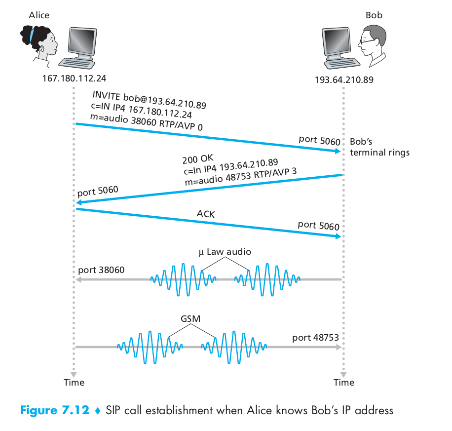
For example, Alice is at her PC and she wants to call Bob, who is also working at his PC. Alice’s and Bob’s PCs are both equipped with SIP-based software for making and receiving phone calls. In this initial example, we’ll assume that Alice knows the IP address of Bob’s PC. Figure 7.12 illustrates the SIP call-establishment process. In Figure 7.12, we see that an SIP session begins when Alice sends Bob an INVITE message, which resembles an HTTP request message. This INVITE message is sent over UDP to the well-known port 5060 for SIP. (SIP messages can also be sent over TCP.) The INVITE message includes an identifier for Bob (bob@193.64.210.89), an indication of Alice’s current IP address, an indication that Alice desires to receive audio, which is to be encoded in format AVP 0 (PCM encoded μ-law) and encapsulated in RTP, and an indication that she wants to receive the RTP packets on port 38060. After receiving Alice’s INVITE message, Bob sends an SIP response message, which resembles an HTTP response message. This response SIP message is also sent to the SIP port 5060. Bob’s response includes a 200 OK as well as an indication of his IP address, his desired encoding and packetization for reception, and his port number to which the audio packets should be sent. Note that in this example Alice and Bob are going to use different audio-encoding mechanisms: Alice is asked to encode her audio with GSM whereas Bob is asked to encode his audio with PCM μ-law. After receiving Bob’s response, Alice sends Bob an SIP acknowledgment message. After this SIP transaction, Bob and Alice can talk. (For visual convenience, Figure 7.12 shows Alice talking after Bob, but in truth they would normally talk at the same time.) Bob will encode and packetize the audio as requested and send the audio packets to port number 38060 at IP address 167.180.112.24. Alice will also encode and packetize the audio as requested and send the audio packets to port number 48753 at IP address 193.64.210.89. In this example, let’s consider what would happen if Bob does not have a PCM μ-law codec for encoding audio. In this case, instead of responding with 200 OK, Bob would likely respond with a 600 Not Acceptable and list in the message all the codecs he can use. Alice would then choose one of the listed codecs and send another INVITE message, this time advertising the chosen codec. Bob could also simply reject the call by sending one of many possible rejection reply codes.

In the example in Figure 7.12, we assumed that Alice’s SIP device knew the IP address where Bob could be contacted. But this assumption is quite unrealistic, not only because IP addresses are often dynamically assigned with DHCP, but also because Bob may have multiple IP devices (for example, different devices for his home, work, and car). So now let us suppose that Alice knows only Bob’s e-mail address, bob@domain.com, and that this same address is used for SIP-based calls. In this case, Alice needs to obtain the IP address of the device that the user bob@domain.com is currently using. To find this out, Alice creates an INVITE message that begins with INVITE bob@domain.com SIP/2.0 and sends this message to an SIP proxy. The proxy will respond with an SIP reply that might include the IP address of the device that bob@domain.com is currently using. Alternatively, the reply might include the IP address of Bob’s voicemail box, or it might include a URL of a Web page (that says “Bob is sleeping. Leave me alone!”). Now, you are probably wondering, how can the proxy server determine the current IP address for bob@domain.com? To answer this question, we need to say a few words about another SIP device, the SIP registrar. Every SIP user has an associated registrar. Whenever a user launches an SIP application on a device, the application sends an SIP register message to the registrar, informing the registrar of its current IP address. It is worth noting that the registrar is analogous to a DNS authoritative name server: The DNS server translates fixed host names to fixed IP addresses; the SIP registrar translates fixed human identifiers (for example, bob@domain.com) to dynamic IP addresses. Often SIP registrars and SIP proxies are run on the same host.

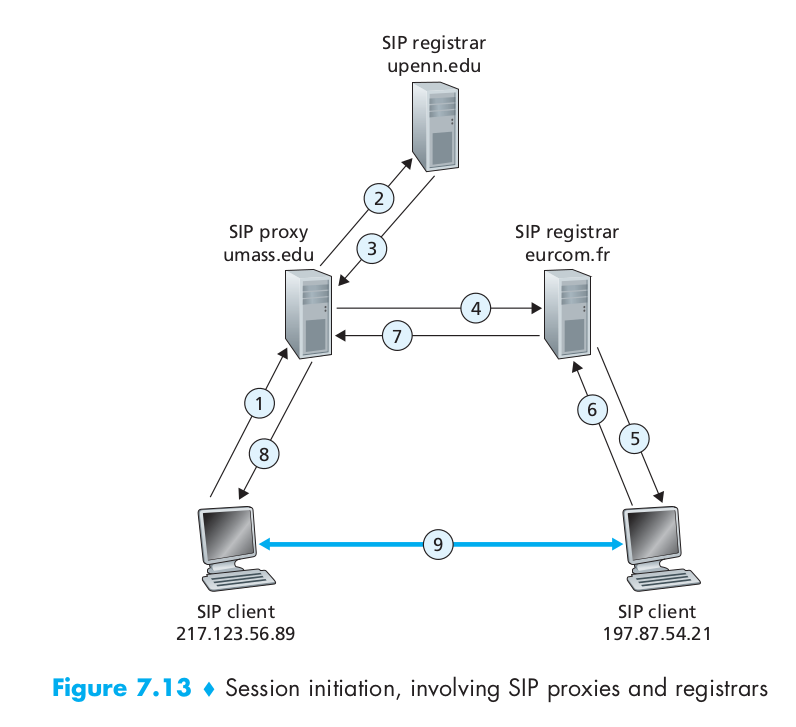
As an example, consider Figure 7.13, in which jim@umass.edu, currently working on 217.123.56.89, wants to initiate a Voice-over-IP (VoIP) session with keith@upenn.edu, currently working on 197.87.54.21. The following steps are taken: (1) Jim sends an INVITE message to the umass SIP proxy. (2) The proxy does a DNS lookup on the SIP registrar upenn.edu (not shown in diagram) and then forwards the message to the registrar server. (3) Because keith@upenn.edu is no longer registered at the upenn registrar, the upenn registrar sends a redirect response, indicating that it should try keith@eurecom.fr. (4) The umass proxy sends an INVITE message to the eurecom SIP registrar. (5) The eurecom registrar knows the IP address of keith@eurecom.fr and forwards the INVITE message to the host 197.87.54.21, which is running Keith’s SIP client. (6–8) An SIP response is sent back through registrars/proxies to the SIP client on 217.123.56.89. (9) Media is sent directly between the two clients. (There is also an SIP acknowledgment message, which is not shown.)

From this simple example, we have learned a number of key characteristics of SIP. First, SIP is an out-of-band protocol: The SIP messages are sent and received in sockets that are different from those used for sending and receiving the media data. Second, the SIP messages themselves are ASCII-readable and resemble HTTP messages. Third, SIP requires all messages to be acknowledged, so it can run over UDP or TCP.