OSI Model Link Layer

• Error-Detection and -Correction Techniques
  • Parity Checks
  • Checksumming Method
  • Cyclic Redundancy Check (CRC)
• Multiple Access Links and Protocols
  • Channel Partitioning Protocols
  • Random Access Protocols
    • Slotted ALOHA
    • Carrier Sense Multiple Access (CDMA)
    • Carrier Sense Multiple Access with Collision Dection (CSMA/CD)
  • Taking Turns Protocols
• Switched Local Area Networks
  • Address Resolution Protocol (ARP)
  • Ethernet
  • Link-Layer Switches
  • Virtual Local Area Networks (VLANs)

We’ll find it convenient in this chapter to refer to any device that runs a link-layer (i.e., layer 2) protocol as a node. Nodes include hosts, routers, switches, and WiFi access points. We will also refer to the communication channels that connect adjacent nodes along the communication path as links.

Although the basic service of any link layer is to move a datagram from one node to an adjacent node over a single communication link, the details of the provided service can vary from one link-layer protocol to the next. Possible services that can be offered by a link-layer protocol include:

• Framing. Almost all link-layer protocols encapsulate each network-layer datagram within a link-layer frame before transmission over the link. A frame consists of a data field, in which the network-layer datagram is inserted, and a number of header fields. The structure of the frame is specified by the link-layer protocol.
• Link access. A medium access control (MAC) protocol specifies the rules by which a frame is transmitted onto the link. For point-to-point links that have a single sender at one end of the link and a single receiver at the other end of the link, the MAC protocol is simple (or nonexistent) – the sender can send a frame whenever the link is idle. The more interesting case is when multiple nodes share a single broadcast link – the so-called multiple access problem. Here, the MAC protocol serves to coordinate the frame transmissions of the many nodes.
• Reliable delivery. When a link-layer protocol provides reliable delivery service, it guarantees to move each network-layer datagram across the link without error. Recall that certain transport-layer protocols (such as TCP) also provide a reliable delivery service. Similar to a transport-layer reliable delivery service, a link-layer reliable delivery service can be achieved with acknowledgments and retransmissions. A link-layer reliable delivery service is often used for links that are prone to high error rates, such as a wireless link, with the goal of correcting an error locally – on the link where the error occurs – rather than forcing an end-to-end retransmission of the data by a transport- or application-layer protocol. However, link-layer reliable delivery can be considered an unnecessary overhead for low bit-error links, including fiber, coax, and many twisted-pair copper links. For this reason, many wired link-layer protocols do not provide a reliable delivery service.
• Error detection and correction. The link-layer hardware in a receiving node can incorrectly decide that a bit in a frame is zero when it was transmitted as a one, and vice versa. Such bit errors are introduced by signal attenuation and electromagnetic noise. Because there is no need to forward a datagram that has an error, many link-layer protocols provide a mechanism to detect such bit errors. This is done by having the transmitting node include error-detection bits in the frame, and having the receiving node perform an error check. The Internet’s transport layer and network layer also provide a limited form of error detection – the Internet checksum. Error detection in the link layer is usually more sophisticated and is implemented in hardware. Error correction is similar to error detection, except that a receiver not only detects when bit errors have occurred in the frame but also determines exactly where in the frame the errors have occurred (and then corrects these errors).

Figure 5.2 shows a typical host architecture. For the most part, the link layer is implemented in a network adapter, also sometimes known as a network interface card (NIC). At the heart of the network adapter is the link-layer controller, usually a single, special-purpose chip that implements many of the link-layer services (framing, link access, error detection, and so on). Thus, much of a link-layer controller’s functionality is implemented in hardware while part of the link layer is implemented in software that runs on the host’s CPU..

Error-Detection and -Correction Techniques

Typically, the data to be protected includes not only the datagram passed down from the network layer for transmission across the link, but also link-level addressing information, sequence numbers, and other fields in the link frame header. Error-detection and -correction techniques allow the receiver to sometimes, but not always, detect that bit errors have occurred. Even with the use of error-detection bits there still may be undetected bit errors.

Parity Checks

Perhaps the simplest form of error detection is the use of a single parity bit. Suppose that the information to be sent, D in Figure 5.4, has d bits. In an even parity scheme, the sender simply includes one additional bit and chooses its value such that the total number of 1s in the d + 1 bits (the original information plus a parity bit) is even. For odd parity schemes, the parity bit value is chosen such that there is an odd number of 1s. Figure 5.4 illustrates an even parity scheme, with the single parity bit being stored in a separate field. Receiver operation is also simple with a single parity bit. The receiver need only count the number of 1s in the received d + 1 bits. If an odd number of 1-valued bits are found with an even parity scheme, the receiver knows that at least one bit error has occurred. More precisely, it knows that some odd number of bit errors have occurred. If an even number of bit errors occur, this would result in an undetected error. If the probability of bit errors is small and errors can be assumed to occur independently from one bit to the next, the probability of multiple bit errors in a packet would be extremely small. In this case, a single parity bit might suffice. However, measurements have shown that, rather than occurring independently, errors are often clustered together in “bursts.”

Figure 5.5 shows a two-dimensional generalization of the single-bit parity scheme. Here, the d bits in D are divided into i rows and j columns. A parity value is computed for each row and for each column. The resulting i + j + 1 parity bits comprise the link-layer frame’s error-detection bits. Figure 5.5 shows an example in which the 1-valued bit in position (2,2) is corrupted and switched to a 0 – an error that is both detectable and correctable at the receiver. The ability of the receiver to both detect and correct errors is known as forward error correction (FEC). These techniques are commonly used in audio storage and playback devices such as audio CDs.

Checksumming Method

In checksumming techniques, the d bits of data in Figure 5.4 are treated as a sequence of k-bit integers. One simple checksumming method is to simply sum these k-bit integers and use the resulting sum as the error-detection bits. The Internet checksum is based on this approach – bytes of data are treated as 16-bit integers and summed. The 1s complement of this sum then forms the Internet checksum that is carried in the segment header. The receiver checks the checksum by taking the 1s complement of the sum of the received data (including the checksum) and checking whether the result is all 1 bits. If any of the bits are 0, an error is indicated. RFC 1071 discusses the Internet checksum algorithm and its implementation in detail. In the TCP and UDP protocols, the Internet checksum is computed over all fields (header and data fields included). In IP the checksum is computed over the IP header (since the UDP or TCP segment has its own checksum).

Cyclic Redundancy Check (CRC)

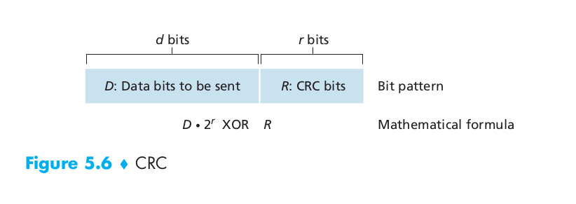
An error-detection technique used widely in today’s computer networks is based on cyclic redundancy check (CRC) codes. CRC codes are also known as polynomial codes, since it is possible to view the bit string to be sent as a polynomial whose coefficients are the 0 and 1 values in the bit string, with operations on the bit string interpreted as polynomial arithmetic. CRC codes operate as follows. Consider the d-bit piece of data, D, that the sending node wants to send to the receiving node. The sender and receiver must first agree on an r + 1 bit pattern, known as a generator, which we will denote as G. We will require that the most significant (leftmost) bit of G be a 1. The key idea behind CRC codes is shown in Figure 5.6. For a given piece of data, D, the sender will choose r additional bits, R, and append them to D such that the resulting d + r bit pattern (interpreted as a binary number) is exactly divisible by G (i.e., has no remainder) using modulo-2 arithmetic. The process of error checking with CRCs is thus simple: The receiver divides the d + r received bits by G. If the remainder is nonzero, the receiver knows that an error has occurred; otherwise the data is accepted as being correct.

Note that the generator is r + b bits if R is r bits.

Multiple Access Links and Protocols

We noted that there are two types of network links: point-to-point links and broadcast links. A point-to-point link consists of a single sender at one end of the link and a single receiver at the other end of the link. Many link-layer protocols have been designed for point-to-point links; the point-to-point protocol (PPP) and high-level data link control (HDLC) are two such protocols. The second type of link, a broadcast link, can have multiple sending and receiving nodes all connected to the same, single, shared broadcast channel. The term broadcast is used here because when any one node transmits a frame, the channel broadcasts the frame and each of the other nodes receives a copy. Ethernet and wireless LANs are examples of broadcast link-layer technologies. Because all nodes are capable of transmitting frames, more than two nodes can transmit frames at the same time. When this happens, all of the nodes receive multiple frames at the same time; that is, the transmitted frames collide at all of the receivers. Typically, when there is a collision, none of the receiving nodes can make any sense of any of the frames that were transmitted; in a sense, the signals of the colliding frames become inextricably tangled together. Thus, all the frames involved in the collision are lost, and the broadcast channel is wasted during the collision interval. In order to ensure that the broadcast channel performs useful work when multiple nodes are active, it is necessary to somehow coordinate the transmissions of the active nodes. This coordination job is the responsibility of the multiple access protocol.

Let’s conclude this overview by noting that, ideally, a multiple access protocol for a broadcast channel of rate R bits per second should have the following desirable characteristics:

1. When only one node has data to send, that node has a throughput of R bps.
2. When M nodes have data to send, each of these nodes has a throughput of R/M bps. This need not necessarily imply that each of the M nodes always has an instantaneous rate of R/M, but rather that each node should have an average transmission rate of R/M over some suitably defined interval of time.
3. The protocol is decentralized; that is, there is no master node that represents a single point of failure for the network.
4. The protocol is simple, so that it is inexpensive to implement.

Channel Partitioning Protocols

Time-division multiplexing (TDM) and frequency-division multiplexing (FDM) are two techniques that can be used to partition a broadcast channel’s bandwidth among all nodes sharing that channel.

As an example, suppose the channel supports N nodes and that the transmission rate of the channel is R bps. TDM divides time into time frames and further divides each time frame into N time slots. Each time slot is then assigned to one of the N nodes. Whenever a node has a packet to send, it transmits the packet’s bits during its assigned time slot in the revolving TDM frame. Typically, slot sizes are chosen so that a single packet can be transmitted during a slot time. TDM is appealing because it eliminates collisions and is perfectly fair: Each node gets a dedicated transmission rate of R/N bps during each frame time. However, it has two major drawbacks. First, a node is limited to an average rate of R/N bps even when it is the only node with packets to send. A second drawback is that a node must always wait for its turn in the transmission sequence – again, even when it is the only node with a frame to send.

While TDM shares the broadcast channel in time, FDM divides the R bps channel into different frequencies (each with a bandwidth of R/N) and assigns each frequency to one of the N nodes. FDM shares both the advantages and drawbacks of TDM. It avoids collisions and divides the bandwidth fairly among the N nodes. However, FDM also shares a principal disadvantage with TDM – a node is limited to a bandwidth of R/N, even when it is the only node with packets to send.

A third channel partitioning protocol is code division multiple access (CDMA). While TDM and FDM assign time slots and frequencies, respectively, to the nodes, CDMA assigns a different code to each node. Each node then uses its unique code to encode the data bits it sends.

Random Access Protocols

In a random access protocol, a transmitting node always transmits at the full rate of the channel, namely, R bps. When there is a collision, each node involved in the collision repeatedly retransmits its frame (that is, packet) until its frame gets through without a collision. But when a node experiences a collision, it doesn’t necessarily retransmit the frame right away. Instead it waits a random delay before retransmitting the frame. Each node involved in a collision chooses independent random delays. Because the random delays are independently chosen, it is possible that one of the nodes will pick a delay that is sufficiently less than the delays of the other colliding nodes and will therefore be able to sneak its frame into the channel without a collision.

Slotted ALOHA

In our description of slotted ALOHA, we assume the following:

• All frames consist of exactly L bits.
• Time is divided into slots of size L/R seconds (that is, a slot equals the time to transmit one frame).
• Nodes start to transmit frames only at the beginnings of slots.
• The nodes are synchronized so that each node knows when the slots begin.
• If two or more frames collide in a slot, then all the nodes detect the collision event before the slot ends.

Let p be a probability, that is, a number between 0 and 1. The operation of slotted ALOHA in each node is simple:

• When the node has a fresh frame to send, it waits until the beginning of the next slot and transmits the entire frame in the slot.
• If there isn’t a collision, the node has successfully transmitted its frame and thus need not consider retransmitting the frame. (The node can prepare a new frame for transmission, if it has one.)
• If there is a collision, the node detects the collision before the end of the slot. The node retransmits its frame in each subsequent slot with probability p until the frame is transmitted without a collision.

Slotted ALOHA would appear to have many advantages. Unlike channel partitioning, slotted ALOHA allows a node to transmit continuously at the full rate, R, when that node is the only active node. (A node is said to be active if it has frames to send.) Slotted ALOHA is also highly decentralized, because each node detects collisions and independently decides when to retransmit. Slotted ALOHA works well when there is only one active node, but how efficient is it when there are multiple active nodes? There are two possible efficiency concerns here. First, when there are multiple active nodes, a certain fraction of the slots will have collisions and will therefore be “wasted.” The second concern is that another fraction of the slots will be empty because all active nodes refrain from transmitting as a result of the probabilistic transmission policy. The only “unwasted” slots will be those in which exactly one node transmits. A slot in which exactly one node transmits is said to be a successful slot.

Therefore the probability a given node has a success is $p(1 – p)^{N - 1}$. Because there are N nodes, the probability that any one of the N nodes has a success is $Np(1 – p)^{N - 1}$. Thus, when there are N active nodes, the efficiency of slotted ALOHA is $Np(1 – p)^{N - 1}$. To obtain the maximum efficiency for N active nodes, we have to find the p that maximizes this expression. And to obtain the maximum efficiency for a large number of active nodes, we take the limit of $Np(1 – p)^{N - 1}$ as N approaches infinity. After performing these calculations, we’ll find that the maximum efficiency of the protocol is given by 1/e = 0.37. That is, when a large number of nodes have many frames to transmit, then (at best) only 37 percent of the slots do useful work. A similar analysis also shows that 37 percent of the slots go empty and 26 percent of slots have collisions.

Carrier Sense Multiple Access (CDMA)

In the networking world, this is called carrier sensing – a node listens to the channel before transmitting. If a frame from another node is currently being transmitted into the channel, a node then waits until it detects no transmissions for a short amount of time and then begins transmission.

In the networking world, this is called collision detection – a transmitting node listens to the channel while it is transmitting. If it detects that another node is transmitting an interfering frame, it stops transmitting and waits a random amount of time before repeating the sense-and-transmit-when-idle cycle.

These two rules are embodied in the family of carrier sense multiple access (CSMA) and CSMA with collision detection (CSMA/CD) protocols.

Figure 5.12 shows a space-time diagram of four nodes (A, B, C, D) attached to a linear broadcast bus. The horizontal axis shows the position of each node in space; the vertical axis represents time.

At time $t_0$, node B senses the channel is idle, as no other nodes are currently transmitting. Node B thus begins transmitting, with its bits propagating in both directions along the broadcast medium. At time $t_1$ ($t_1$ > $t_0$ ), node D has a frame to send. Although node B is currently transmitting at time $t_1$, the bits being transmitted by B have yet to reach D, and thus D senses the channel idle at $t_1$. In accordance with the CSMA protocol, D thus begins transmitting its frame. A short time later, B’s transmission begins to interfere with D’s transmission at D. From Figure 5.12, it is evident that the end-to-end channel propagation delay of a broadcast channel – the time it takes for a signal to propagate from one of the nodes to another – will play a crucial role in determining its performance. The longer this propagation delay, the larger the chance that a carrier-sensing node is not yet able to sense a transmission that has already begun at another node in the network.

Carrier Sense Multiple Access with Collision Dection (CSMA/CD)

Before analyzing the CSMA/CD protocol, let us now summarize its operation from the perspective of an adapter (in a node) attached to a broadcast channel:

1. The adapter obtains a datagram from the network layer, prepares a link-layer frame, and puts the frame adapter buffer.
2. If the adapter senses that the channel is idle (that is, there is no signal energy entering the adapter from the channel), it starts to transmit the frame. If, on the other hand, the adapter senses that the channel is busy, it waits until it senses no signal energy and then starts to transmit the frame.
3. While transmitting, the adapter monitors for the presence of signal energy coming from other adapters using the broadcast channel.
4. If the adapter transmits the entire frame without detecting signal energy from other adapters, the adapter is finished with the frame. If, on the other hand, the adapter detects signal energy from other adapters while transmitting, it aborts the transmission (that is, it stops transmitting its frame).
5. After aborting, the adapter waits a random amount of time and then returns to step 2.

What is a good interval of time from which to choose the random backoff time? If the interval is large and the number of colliding nodes is small, nodes are likely to wait a large amount of time (with the channel remaining idle) before repeating the sense-and-transmit-when-idle step. On the other hand, if the interval is small and the number of colliding nodes is large, it’s likely that the chosen random values will be nearly the same, and transmitting nodes will again collide. What we’d like is an interval that is short when the number of colliding nodes is small, and long when the number of colliding nodes is large. The binary exponential backoff algorithm, used in Ethernet as well as in DOCSIS cable network multiple access protocols, elegantly solves this problem. Specifically, when transmitting a frame that has already experienced n collisions, a node chooses the value of K at random from {$0,1,2, \ldots 2^{n}-1$}. Thus, the more collisions experienced by a frame, the larger the interval from which K is chosen. For Ethernet, the actual amount of time a node waits is K * 512 bit times (i.e., K times the amount of time needed to send 512 bits into the Ethernet) and the maximum value that n can take is capped at 10.

We define the efficiency of CSMA/CD to be the long-run fraction of time during which frames are being transmitted on the channel without collisions when there is a large number of active nodes, with each node having a large number of frames to send. In order to present a closed-form approximation of the efficiency of Ethernet, let $d_{\text {prop }}$ denote the maximum time it takes signal energy to propagate between any two adapters. Let $d_{\text {trans }}$ be the time to transmit a maximum-size frame. Here we simply state the following approximation:

Taking Turns Protocols

As with random access protocols, there are dozens of taking-turns protocols, and each one of these protocols has many variations. We’ll discuss two of the more important protocols here.

The first one is the polling protocol. The polling protocol requires one of the nodes to be designated as a master node. The master node polls each of the nodes in a round-robin fashion. The polling protocol eliminates the collisions and empty slots that plague random access protocols. This allows polling to achieve a much higher efficiency. But it also has a few drawbacks. The first drawback is that the protocol introduces a polling delay – the amount of time required to notify a node that it can transmit. If, for example, only one node is active, then the node will transmit at a rate less than R bps, as the master node must poll each of the inactive nodes in turn each time the active node has sent its maximum number of frames. The second drawback, which is potentially more serious, is that if the master node fails, the entire channel becomes inoperative.

The second taking-turns protocol is the token-passing protocol. In this protocol there is no master node. A small, special-purpose frame known as a token is exchanged among the nodes in some fixed order. For example, node 1 might always send the token to node 2, node 2 might always send the token to node 3, and node N might always send the token to node 1. When a node receives a token, it holds onto the token only if it has some frames to transmit; otherwise, it immediately forwards the token to the next node. If a node does have frames to transmit when it receives the token, it sends up to a maximum number of frames and then forwards the token to the next node. Token passing is decentralized and highly efficient. But it has its problems as well. For example, the failure of one node can crash the entire channel. Or if a node accidentally neglects to release the token, then some recovery procedure must be invoked to get the token back in circulation.

Switched Local Area Networks

Address Resolution Protocol (ARP)

In truth, it is not hosts and routers that have link-layer addresses but rather their adapters (that is, network interfaces) that have link-layer addresses. A host or router with multiple network interfaces will thus have multiple link-layer addresses associated with it, just as it would also have multiple IP addresses associated with it. It’s important to note, however, that link-layer switches do not have link-layer addresses associated with their interfaces that connect to hosts and routers. A link-layer address is variously called a LAN address, a physical address, or a MAC address. Sometimes a sending adapter does want all the other adapters on the LAN to receive and process the frame it is about to send. In this case, the sending adapter inserts a special MAC broadcast address into the destination address field of the frame. For LANs that use 6-byte addresses (such as Ethernet and 802.11), the broadcast address is a string of 48 consecutive 1s (that is, FF-FF-FF-FF-FF-FF in hexadecimal notation).

Because there are both network-layer addresses (for example, Internet IP addresses) and link-layer addresses (that is, MAC addresses), there is a need to translate between them. For the Internet, this is the job of the Address Resolution Protocol (ARP) [RFC 826]. Now suppose that the host with IP address 222.222.222.220 wants to send an IP datagram to host 222.222.222.222. To send a datagram, the source must give its adapter not only the IP datagram but also the MAC address for destination 222.222.222.222. The sending adapter will then construct a link-layer frame containing the destination’s MAC address and send the frame into the LAN. The important question addressed in this section is, How does the sending host determine the MAC address for the destination host with IP address 222.222.222.222? As you might have guessed, it uses ARP. An ARP module in the sending host takes any IP address on the same LAN as input, and returns the corresponding MAC address. In the example at hand, sending host 222.222.222.220 provides its ARP module the IP address 222.222.222.222, and the ARP module returns the corresponding MAC address 49-BD-D2-C7-56-2A. Though DNS is similar to the ARP, one important difference between the two resolvers is that DNS resolves host names for hosts anywhere in the Internet, whereas ARP resolves IP addresses only for hosts and router interfaces on the same subnet.

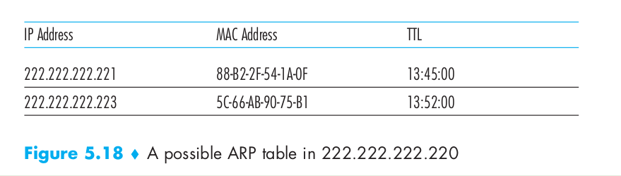
Each host and router has an ARP table in its memory, which contains mappings of IP addresses to MAC addresses. Figure 5.18 shows what an ARP table in host 222.222.222.220 might look like. The ARP table also contains a time-to-live (TTL) value, which indicates when each mapping will be deleted from the table. Note that a table does not necessarily contain an entry for every host and router on the subnet; some may have never been entered into the table, and others may have expired. A typical expiration time for an entry is 20 minutes from when an entry is placed in an ARP table. If source host want to send a datagram to a destination host whose IP address is not included inside the ARP table, the source host will try to get the MAC address with the destination IP address. First, the sender constructs a special packet called an ARP packet. An ARP packet has several fields, including the sending and receiving IP and MAC addresses. Both ARP query and response packets have the same format. The purpose of the ARP query packet is to query all the other hosts and routers on the subnet to determine the MAC address corresponding to the IP address that is being resolved. Returning to our example, 222.222.222.220 passes an ARP query packet to the adapter along with an indication that the adapter should send the packet to the MAC broadcast address, namely, FF-FF-FF-FF-FF-FF. The adapter encapsulates the ARP packet in a link-layer frame, uses the broadcast address for the frame’s destination address, and transmits the frame into the subnet. The frame containing the ARP query is received by all the other adapters on the subnet, and (because of the broadcast address) each adapter passes the ARP packet within the frame up to its ARP module. Each of these ARP modules checks to see if its IP address matches the destination IP address in the ARP packet. The one with a match sends back to the querying host a response ARP packet with the desired mapping. The querying host 222.222.222.220 can then update its ARP table and send its IP datagram, encapsulated in a link-layer frame whose destination MAC is that of the host or router responding to the earlier ARP query.

If a host want to send a datagram off the subnet, now let’s examine how a host on Subnet 1 would send a datagram to a host on Subnet 2. Specifically, suppose that host 111.111.111.111 wants to send an IP datagram to a host 222.222.222.222. In order for a datagram to go from 111.111.111.111 to a host on Subnet 2, the datagram must first be sent to the router interface 111.111.111.110, which is the IP address of the first-hop router on the path to the final destination. Thus, the appropriate MAC address for the frame is the address of the adapter for router interface 111.111.111.110, namely, E6-E9-00-17-BB-4B. How does the sending host acquire the MAC address for 111.111.111.110? By using ARP, of course! Once the sending adapter has this MAC address, it creates a frame (containing the datagram addressed to 222.222.222.222) and sends the frame into Subnet 1. The router adapter on Subnet 1 sees that the link-layer frame is addressed to it, and therefore passes the frame to the network layer of the router. The IP datagram has successfully been moved from source host to the router. But we are not finished. We still have to move the datagram from the router to the destination. The router now has to determine the correct interface on which the datagram is to be forwarded. This is done by consulting a forwarding table in the router. The forwarding table tells the router that the datagram is to be forwarded via router interface 222.222.222.220. This interface then passes the datagram to its adapter, which encapsulates the datagram in a new frame and sends the frame into Subnet 2. This time, the destination MAC address of the frame is indeed the MAC address of the ultimate destination. And how does the router obtain this destination MAC address? From ARP, of course!

Ethernet

Let’s now examine the six fields of the Ethernet frame, as shown in Figure 5.20.

• Data field (46 to 1,500 bytes). This field carries the IP datagram. The maximum transmission unit (MTU) of Ethernet is 1,500 bytes. This means that if the IP datagram exceeds 1,500 bytes, then the host has to fragment the datagram. The minimum size of the data field is 46 bytes. This means that if the IP datagram is less than 46 bytes, the data field has to be “stuffed” to fill it out to 46 bytes. When stuffing is used, the data passed to the network layer contains the stuffing as well as an IP datagram. The network layer uses the length field in the IP datagram header to remove the stuffing.
• Destination address (6 bytes). This field contains the MAC address of the destination adapter, BB-BB-BB-BB-BB-BB. When adapter B receives an Ethernet frame whose destination address is either BB-BB-BB-BB-BB-BB or the MAC broadcast address, it passes the contents of the frame’s data field to the network layer; if it receives a frame with any other MAC address, it discards the frame.
• Source address (6 bytes). This field contains the MAC address of the adapter that transmits the frame onto the LAN, in this example, AA-AA-AA-AA-AA-AA.
• Type field (2 bytes). The type field permits Ethernet to multiplex network-layer protocols. To understand this, we need to keep in mind that hosts can use other network-layer protocols besides IP. In fact, a given host may support multiple network-layer protocols using different protocols for different applications. For this reason, when the Ethernet frame arrives at adapter B, adapter B needs to know to which network-layer protocol it should pass (that is, demultiplex) the contents of the data field. IP and other network-layer protocols (for example, Novell IPX or AppleTalk) each have their own, standardized type number. Furthermore, the ARP protocol (discussed in the previous section) has its own type number, and if the arriving frame contains an ARP packet (i.e., has a type field of 0806 hexadecimal), the ARP packet will be demultiplexed up to the ARP protocol. Note that the type field is analogous to the protocol field in the network-layer datagram and the port-number fields in the transport-layer segment; all of these fields serve to glue a protocol at one layer to a protocol at the layer above.
• Cyclic redundancy check (CRC) (4 bytes). The purpose of the CRC field is to allow the receiving adapter, adapter B, to detect bit errors in the frame.
• Preamble (8 bytes). The Ethernet frame begins with an 8-byte preamble field. Each of the first 7 bytes of the preamble has a value of 10101010; the last byte is 10101011. The first 7 bytes of the preamble serve to “wake up” the receiving adapters and to synchronize their clocks to that of the sender’s clock. Why should the clocks be out of synchronization? Keep in mind that adapter A aims to transmit the frame at 10 Mbps, 100 Mbps, or 1 Gbps, depending on the type of Ethernet LAN. However, because nothing is absolutely perfect, adapter A will not transmit the frame at exactly the target rate; there will always be some drift from the target rate, a drift which is not known a priori by the other adapters on the LAN. A receiving adapter can lock onto adapter A’s clock simply by locking onto the bits in the first 7 bytes of the preamble. The last 2 bits of the eighth byte of the preamble (the first two consecutive 1s) alert adapter B that the “important stuff” is about to come.

All of the Ethernet technologies provide connectionless service to the network layer. That is, when adapter A wants to send a datagram to adapter B, adapter A encapsulates the datagram in an Ethernet frame and sends the frame into the LAN, without first handshaking with adapter B. This layer-2 connectionless service is analogous to IP’s layer-3 datagram service and UDP’s layer-4 connectionless service. Ethernet technologies provide an unreliable service to the network layer. Specifically, when adapter B receives a frame from adapter A, it runs the frame through a CRC check, but neither sends an acknowledgment when a frame passes the CRC check nor sends a negative acknowledgment when a frame fails the CRC check. When a frame fails the CRC check, adapter B simply discards the frame. Thus, adapter A has no idea whether its transmitted frame reached adapter B and passed the CRC check. This lack of reliable transport (at the link layer) helps to make Ethernet simple and cheap. But it also means that the stream of datagrams passed to the network layer can have gaps.

Link-Layer Switches

The role of the switch is to receive incoming link-layer frames and forward them onto outgoing links. We’ll see that the switch itself is transparent to the hosts and routers in the subnet; that is, a host/router addresses a frame to another host/router (rather than addressing the frame to the switch) and happily sends the frame into the LAN, unaware that a switch will be receiving the frame and forwarding it.

Filtering is the switch function that determines whether a frame should be forwarded to some interface or should just be dropped. Forwarding is the switch function that determines the interfaces to which a frame should be directed, and then moves the frame to those interfaces. Switch filtering and forwarding are done with a switch table. The switch table contains entries for some, but not necessarily all, of the hosts and routers on a LAN. An entry in the switch table contains (1) a MAC address, (2) the switch interface that leads toward that MAC address, and (3) the time at which the entry was placed in the table. Although this description of frame forwarding may sound similar to our discussion of datagram forwarding, we’ll see shortly that there are important differences.

One important difference is that switches forward packets based on MAC addresses rather than on IP addresses. We will also see that a switch table is constructed in a very different manner from a router’s forwarding table. To understand how switch filtering and forwarding work, suppose a frame with destination address DD-DD-DD-DD-DD-DD arrives at the switch on interface x. The switch indexes its table with the MAC address DD-DD-DD-DD-DD-DD. There are three possible cases:

• There is no entry in the table for DD-DD-DD-DD-DD-DD. In this case, the switch forwards copies of the frame to the output buffers preceding all interfaces except for interface x. In other words, if there is no entry for the destination address, the switch broadcasts the frame.
• There is an entry in the table, associating DD-DD-DD-DD-DD-DD with interface x. In this case, the frame is coming from a LAN segment that contains adapter DD-DD-DD-DD-DD-DD. There being no need to forward the frame to any of the other interfaces, the switch performs the filtering function by discarding the frame.
• There is an entry in the table, associating DD-DD-DD-DD-DD-DD with interface y != x. In this case, the frame needs to be forwarded to the LAN segment attached to interface y. The switch performs its forwarding function by putting the frame in an output buffer that precedes interface y.

A switch has the wonderful property (particularly for the already-overworked network administrator) that its table is built automatically, dynamically, and autonomously – without any intervention from a network administrator or from a configuration protocol. In other words, switches are self-learning. This capability is accomplished as follows:

1. The switch table is initially empty.
2. For each incoming frame received on an interface, the switch stores in its table (1) the MAC address in the frame’s source address field, (2) the interface from which the frame arrived, and (3) the current time. In this manner the switch records in its table the LAN segment on which the sender resides. If every host in the LAN eventually sends a frame, then every host will eventually get recorded in the table.
3. The switch deletes an address in the table if no frames are received with that address as the source address after some period of time (the aging time). In this manner, if a PC is replaced by another PC (with a different adapter), the MAC address of the original PC will eventually be purged from the switch table.

Switches are plug-and-play devices because they require no intervention from a network administrator or user. A network administrator wanting to install a switch need do nothing more than connect the LAN segments to the switch interfaces. The administrator need not configure the switch tables at the time of installation or when a host is removed from one of the LAN segments. Switches are also full-duplex, meaning any switch interface can send and receive at the same time.

Let’s now consider Link-Layer switch’s features and properties.

• Elimination of collisions. In a LAN built from switches (and without hubs), there is no wasted bandwidth due to collisions! The switches buffer frames and never transmit more than one frame on a segment at any one time. As with a router, the maximum aggregate throughput of a switch is the sum of all the switch interface rates. Thus, switches provide a significant performance improvement over LANs with broadcast links.
• Heterogeneous links. Because a switch isolates one link from another, the different links in the LAN can operate at different speeds and can run over different media. Thus, a switch is ideal for mixing legacy equipment with new equipment.
• Management. In addition to providing enhanced security (see sidebar on Focus on Security), a switch also eases network management. For example, if an adapter malfunctions and continually sends Ethernet frames (called a jabbering adapter), a switch can detect the problem and internally disconnect the malfunctioning adapter. With this feature, the network administrator need not get out of bed and drive back to work in order to correct the problem. Similarly, a cable cut disconnects only that host that was using the cut cable to connect to the switch. In the days of coaxial cable, many a network manager spent hours “walking the line” (or more accurately, “crawling the floor”) to find the cable break that brought down the entire network. Switches also gather statistics on bandwidth usage, collision rates, and traffic types, and make this information available to the network manager. This information can be used to debug and correct problems, and to plan how the LAN should evolve in the future.

Given that both switches and routers are candidates for interconnection devices, what are the pros and cons of the two approaches? First consider the pros and cons of switches.

As mentioned above, switches are plug-and-play, a property that is cherished by all the overworked network administrators of the world. Switches can also have relatively high filtering and forwarding rates. Switches have to process frames only up through layer 2, whereas routers have to process datagrams up through layer 3. On the other hand, to prevent the cycling of broadcast frames, the active topology of a switched network is restricted to a spanning tree. Also, a large switched network would require large ARP tables in the hosts and routers and would generate substantial ARP traffic and processing. Furthermore, switches are susceptible to broadcast storms – if one host goes haywire and transmits an endless stream of Ethernet broadcast frames, the switches will forward all of these frames, causing the entire network to collapse.

Now consider the pros and cons of routers. Because network addressing is often hierarchical (and not flat, as is MAC addressing), packets do not normally cycle through routers even when the network has redundant paths. Thus, packets are not restricted to a spanning tree and can use the best path between source and destination. Because routers do not have the spanning tree restriction, they have allowed the Internet to be built with a rich topology that includes, for example, multiple active links between Europe and North America. Another feature of routers is that they provide firewall protection against layer-2 broadcast storms. Perhaps the most significant drawback of routers, though, is that they are not plug-and-play – they and the hosts that connect to them need their IP addresses to be configured. Also, routers often have a larger per-packet processing time than switches, because they have to process up through the layer-3 fields. Typically, small networks consisting of a few hundred hosts have a few LAN segments. Switches suffice for these small networks, as they localize traffic and increase aggregate throughput without requiring any configuration of IP addresses. But larger networks consisting of thousands of hosts typically include routers within the network (in addition to switches). The routers provide a more robust isolation of traffic, control broadcast storms, and use more “intelligent” routes among the hosts in the network.

When a host is connected to a switch, it typically only receives frames that are being explicity sent to it. For example, consider a switched LAN. When host A sends a frame to host B, and there is an entry for host B in the switch table, then the switch will forward the frame only to host B. If host C happens to be running a sniffer, host C will not be able to sniff this A-to-B frame. Thus, in a switched-LAN environment (in contrast to a broadcast link environment such as 802.11 LANs or hub–based Ethernet LANs), it is more difficult for an attacker to sniff frames. However, because the switch broadcasts frames that have destination addresses that are not in the switch table, the sniffer at C can still sniff some frames that are not explicitly addressed to C. Furthermore, a sniffer will be able sniff all Ethernet broadcast frames with broadcast destination address FF–FF–FF–FF–FF–FF. A well-known attack against a switch, called switch poisoning, is to send tons of packets to the switch with many different bogus source MAC addresses, thereby filling the switch table with bogus entries and leaving no room for the MAC addresses of the legitimate hosts. This causes the switch to broadcast most frames, which can then be picked up by the sniffer. As this attack is rather involved even for a sophisticated attacker, switches are significantly less vulnerable to sniffing than are hubs and wireless LANs.

Virtual Local Area Networks (VLANs)

As the name suggests, a switch that supports VLANs allows multiple virtual local area networks to be defined over a single physical local area network infrastructure. Hosts within a VLAN communicate with each other as if they (and no other hosts) were connected to the switch. In a port-based VLAN, the switch’s ports (interfaces) are divided into groups by the network manager. Each group constitutes a VLAN, with the ports in each VLAN forming a broadcast domain (i.e., broadcast traffic from one port can only reach other ports in the group). Figure 5.25 shows a single switch with 16 ports. Ports 2 to 8 belong to the EE VLAN, while ports 9 to 15 belong to the CS VLAN (ports 1 and 16 are unassigned). EE and CS VLAN frames are isolated from each other, and if the user at switch port 8 joins the CS Department, the network operator simply reconfigures the VLAN software so that port 8 is now associated with the CS VLAN. How can traffic from the EE Department be sent to the CS Department? One way to handle this would be to connect a VLAN switch port (e.g., port 1 in Figure 5.25) to an external router and configure that port to belong both the EE and CS VLANs. In this case, even though the EE and CS departments share the same physical switch, the logical configuration would look as if the EE and CS departments had separate switches connected via a router. An IP datagram going from the EE to the CS department would first cross the EE VLAN to reach the router and then be forwarded by the router back over the CS VLAN to the CS host. Fortunately, switch vendors make such configurations easy for the network manager by building a single device that contains both a VLAN switch and a router, so a separate external router is not needed.

Let’s now suppose that rather than having a separate Computer Engineering department, some EE and CS faculty are housed in a separate building, where they need network access, and they’d like to be part of their department’s VLAN. Figure 5.26 shows a second 8-port switch, where the switch ports have been defined as belonging to the EE or the CS VLAN, as needed. But how should these two switches be interconnected? One easy solution would be to define a port belonging to the CS VLAN on each switch (similarly for the EE VLAN) and to connect these ports to each other, as shown in Figure 5.26(a). This solution doesn’t scale, however, since N VLANS would require N ports on each switch simply to interconnect the two switches.

A more scalable approach to interconnecting VLAN switches is known as VLAN trunking. In the VLAN trunking approach shown in Figure 5.26(b), a special port on each switch (port 16 on the left switch and port 1 on the right switch) is configured as a trunk port to interconnect the two VLAN switches. The trunk port belongs to all VLANs, and frames sent to any VLAN are forwarded over the trunk link to the other switch. But this raises yet another question: How does a switch know that a frame arriving on a trunk port belongs to a particular VLAN? The IEEE has defined an extended Ethernet frame format, 802.1Q, for frames crossing a VLAN trunk. As shown in Figure 5.27, the 802.1Q frame consists of the standard Ethernet frame with a four-byte VLAN tag added into the header that carries the identity of the VLAN to which the frame belongs. The VLAN tag is added into a frame by the switch at the sending side of a VLAN trunk, parsed, and removed by the switch at the receiving side of the trunk. The VLAN tag itself consists of a 2-byte Tag Protocol Identifier (TPID) field (with a fixed hexadecimal value of 81-00), a 2-byte Tag Control Information field that contains a 12-bit VLAN identifier field, and a 3-bit priority field that is similar in intent to the IP datagram TOS field.