In this chapter we consider file organizations that are excellent for equality selections. The basic idea is to use a hashing function, which maps values in a search field into a range of bucket numbers to find the page on which a desired data entry belongs. We use a simple scheme called Static Hashing to introduce the idea. This scheme, like ISAM, suffers from the problem of long overflow chains, which can affect performance. Two solutions to the problem are presented. The Extendible Hashing scheme uses a directory to support inserts and deletes efficiently with no overflow pages. The Linear Hashing scheme uses a clever policy for creating new buckets and supports inserts and deletes efficiently without the use of a directory. Although overflow pages are used, the length of overflow chains is rarely more than two. Hash-based indexing techniques cannot support range searches, unfortunately. tree-based indexing techniques can support range searches efficiently and are almost as good as hash-based indexing for equality selections. Thus, many commercial systems choose to support only tree-based indexes. Nonetheless, hashing techniques prove to be very useful in implementing relational operations such as joins. In particular, the Index Nested Loops join method generates many equality selection queries, and the difference in cost between a hash-based index and a tree-based index can become significant in this context.
Static Hashing
The Static Hashing scheme is illustrated in Figure 11.1. The pages containing the data can be viewed as a collection of buckets, with one primary page and possibly additional overflow pages per bucket. A file consists of buckets 0 through N - 1, with one primary page per bucket initially. Buckets contain data entries, which can be any of the three alternatives.

To search for a data entry, we apply a hash function h to identify the bucket to which it belongs and then search this bucket. To speed the search of a bucket, we can maintain data entries in sorted order by search key value; in this chapter, we do not sort entries, and the order of entries within a bucket has no significance. To insert a data entry, we use the hash function to identify the correct bucket and then put the data entry there. If there is no space for this data entry, we allocate a new overflow page, put the data entry on this page, and add the page to the overflow chain of the bucket. To delete a data entry, we use the hashing function to identify the correct bucket, locate the data entry by searching the bucket, and then remove it. If this data entry is the last in an overflow page, the overflow page is removed from the overflow chain of the bucket and added to a list of free pages.
The hash function is an important component of the hashing approach. It must distribute values in the domain of the search field uniformly over the collection of buckets. If we have N buckets, numbered 0 through N ~ 1, a hash function h of the form h(value) = (a * value + b) works well in practice. (The bucket identified is h(value) mod N.) The constants a and b can be chosen to ‘tune’ the hash function. Since the number of buckets in a Static Hashing file is known when the file is created, the primary pages can be stored on successive disk pages. Hence, a search ideally requires just one disk I/O, and insert and delete operations require two I/Os (read and write the page), although the cost could be higher in the presence of overflow pages. As the file grows, long overflow chains can develop. Since searching a bucket requires us to search (in general) all pages in its overflow chain, it is easy to see how performance can deteriorate. By initially keeping pages 80 percent full, we can avoid overflow pages if the file does not grow too much, but in general the only way to get rid of overflow chains is to create a new file with more buckets. The main problem with Static Hashing is that the number of buckets is fixed. If a file shrinks greatly, a lot of space is wasted; more important, if a file grows a lot, long overflow chains develop, resulting in poor performance. Therefore, Static Hashing can be compared to the ISAM structure, which can also develop long overflow chains in case of insertions to the same leaf. Static Hashing also has the same advantages as ISAM with respect to concurrent access. One simple alternative to Static Hashing is to periodically ‘rehash’ the file to restore the ideal situation (no overflow chains, about 80 percent occupancy). However, rehashing takes time and the index cannot be used while rehashing is in progress. Another alternative is to use dynamic hashing techniques such as Extendible and Linear Hashing, which deal with inserts and deletes gracefully.
Extendible Hashing
To understand Extendible Hashing, let us begin by considering a Static Hashing file. If we have to insert a new data entry into a full bucket, we need to add an overflow page. If we do not want to add overflow pages, one solution is to reorganize the file at this point by doubling the number of buckets and redistributing the entries across the new set of buckets. This solution suffers from one major defect–the entire file has to be read, and twice as many pages have to be written to achieve the reorganization. This problem, however, can be overcome by a simple idea: Use a directory of pointers to buckets, and double the size of the number of buckets by doubling just the directory and splitting only the bucket that overflowed.
To understand the idea, consider the sample file shown in Figure 11.2. The directory consists of an array of size 4, with each element being a pointer to a bucket. (The global depth and local depth fields are discussed shortly, ignore them for now.) To locate a data entry, we apply a hash function to the search field and take the last 2 bits of its binary representation to get a number between 0 and 3. The pointer in this array position gives us the desired bucket; we assume that each bucket can hold four data entries. Therefore, to locate a data entry with hash value 5 (binary 101), we look at directory element 01 and follow the pointer to the data page (bucket B in the figure).

To insert a data entry, we search to find the appropriate bucket. For example, to insert a data entry with hash value 13 (denoted as 13*), we examine directory element 01 and go to the page containing data entries 1*, 5*, and 21*. Since the page has space for an additional data entry, we are done after we insert the entry (Figure 11.3).

Next, let us consider insertion of a data entry into a full bucket. The essence of the Extendible Hashing idea lies in how we deal with this case. Consider the insertion of data entry 20* (binary 10100). Looking at directory element 00, we are led to bucket A, which is already full. We must first split the bucket by allocating a new bucket and redistributing the contents (including the new entry to be inserted) across the old bucket and its ‘split image.’ To redistribute entries across the old bucket and its split image, we consider the last three bits of h(T); the last two bits are 00, indicating a data entry that belongs to one of these two buckets, and the third bit discriminates between these buckets. The redistribution of entries is illustrated in Figure 11.4.

Note a problem that we must now resolve–we need three bits to discriminate between two of our data pages (A and A2), but the directory has only enough slots to store all two-bit patterns. The solution is to double the directory. Elements that differ only in the third bit from the end are said to ‘correspond’: corresponding elements of the directory point to the same bucket with the exception of the elements corresponding to the split bucket. In our example, bucket a was split; so, new directory element 000 points to one of the split versions and new element 100 points to the other. The sample file after completing all steps in the insertion of 20* is shown in Figure 11.5.

Therefore, doubling the file requires allocating a new bucket page, writing both this page and the old bucket page that is being split, and doubling the directory array. The directory is likely to be much smaller than the file itself because each element is just a page-id, and can be doubled by simply copying it over (and adjusting the elements for the split buckets). The cost of doubling is now quite acceptable.
We observe that the basic technique used in Extendible Hashing is to treat the result of applying a hash function h as a binary number and interpret the last d bits, where d depends on the size of the directory, as an offset into the directory. In our example, d is originally 2 because we only have four buckets; after the split, d becomes 3 because we now have eight buckets. A corollary is that, when distributing entries across a bucket and its split image, we should do so on the basis of the d th bit. (Note how entries are redistributed in our example; see Figure 11.5.) The number d, called the global depth of the hashed file, is kept as part of the header of the file. It is used every time we need to locate a data entry. An important point that arises is whether splitting a bucket necessitates a directory doubling. Consider our example, as shown in Figure 11.5. If we now insert 9*, it belongs in bucket B; this bucket is already full. We can deal with this situation by splitting the bucket and using directory elements 001 and 101 to point to the bucket and its split image, as shown in Figure 11.6. Hence, a bucket split does not necessarily require a directory doubling. However, if either bucket A or A2 grows full and an insert then forces a bucket split, we are forced to double the directory again.

To differentiate between these cases and determine whether a directory doubling is needed, we maintain a local depth for each bucket. If a bucket whose local depth is equal to the global depth is split, the directory must be doubled. Going back to the example, when we inserted 9* into the index shown in Figure 11.5, it belonged to bucket B with local depth 2, whereas the global depth was 3. Even though the bucket was split, the directory did not have to be doubled. Buckets A and A2, on the other hand, have local depth equal to the global depth, and, if they grow full and are split, the directory must then be doubled. Initially, all local depths are equal to the global depth (which is the number of bits needed to express the total number of buckets). We increment the global depth by 1 each time the directory doubles, of course. Also, whenever a bucket is split (whether or not the split leads to a directory doubling), we increment by 1 the local depth of the split bucket and assign this same (incremented) local depth to its (newly created) split image. Intuitively, if a bucket has local depth l, the hash values of data entries in it agree on the last l bits; further, no data entry in any other bucket of the file has a hash value with the same last l bits. A total of $2^{d - l}$ directory elements point to a bucket with local depth l; if d = l, exactly one directory element points to the bucket and splitting such a bucket requires directory doubling. A final point to note is that we can also use the first d bits (the most significant bits) instead of the last d (least significant bits), but in practice the last d bits are used. The reason is that a directory can then be doubled simply by copying it.
In summary, a data entry can be located by computing its hash value, taking the last d bits, and looking in the bucket pointed to by this directory element. For inserts, the data entry is placed in the bucket to which it belongs and the bucket is split if necessary to make space. A bucket split leads to an increase in the local depth and, if the local depth becomes greater than the global depth as a result to a directory doubling (and an increase in the global depth) as well. For deletes, the data entry is located and removed. If the delete leaves the bucket empty, it can be merged with its split image, although this step is often omitted in practice. Merging buckets decreases the local depth. If each directory element points to the same bucket as its split image (i.e., 0 and $2^{d - 1}$ point to the same bucket, namely, A; 1 and $2^{d - 1} + 1$ point to the same bucket, namely, B, which mayor may not be identical to A; etc.), we can halve the directory and reduce the global depth, although this step is not necessary for correctness. The insertion examples can be worked out backwards as examples of deletion. (Start with the structure shown after an insertion and delete the inserted element. In each case the original structure should be the result.) If the directory fits in memory, an equality selection can be answered in a single disk access, as for Static Hashing (in the absence of overflow pages), but otherwise, two disk I/Os are needed. As a typical example, a 100MB file with 100 bytes per data entry and a page size of 4KB contains 1 million data entries and only about 25,000 elements in the directory. (Each page/bucket contains roughly 40 data entries, and we have one directory element per bucket.) Thus, although equality selections can be twice as slow as for Static Hashing files, chances are high that the directory will fit in memory and performance is the same as for Static Hashing files. On the other hand, the directory grows in spurts and can become large for skewed data distributions (where our assumption that data pages contain roughly equal numbers of data entries is not valid). In the context of hashed files, in a skewed data distribution the distribution of hash values of search field values (rather than the distribution of search field values themselves) is skewed (very ‘bursty’ or nonuniform). Even if the distribution of search values is skewed, the choice of a good hashing function typically yields a fairly uniform distribution of hash values; skew is therefore not a problem in practice. Further, collisions, or data entries with the same hash value, cause a problem and must be handled specially: When more data entries then will fit on a page have the same hash value, we need overflow pages.
Linear Hashing
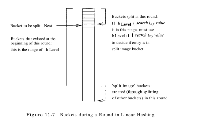
Linear Hashing is a dynamic hashing technique, like Extendible Hashing, adjusting gracefully to inserts and deletes. In contrast to Extendible Hashing, it does not require a directory, deals naturally with collisions, and offers a lot of flexibility with respect to the timing of bucket splits (allowing us to trade off slightly greater overflow chains for higher average space utilization). If the data distribution is very skewed, however, overflow chains could cause Linear Hashing performance to be worse than that of Extendible Hashing. The scheme utilizes a family of hash functions $h_0, h_1, h_2$, … , with the property that each function’s range is twice that of its predecessor. That is, if $h_i$ maps a data entry into one of M buckets, $h_(i + 1)$ maps a data entry into one of 2M buckets. Such a family is typically obtained by choosing a hash function h and an initial number N of buckets and defining $h_i(value) = h(value) mod (2^i N)$. If N is chosen to be a power of 2, then we apply h and look at the last $d_i$ bits; $d_0$ is the number of bits needed to represent N, and $d_i = d_0 + i$. Typically we choose h to be a function that maps a data entry to some integer. Suppose that we set the initial number N of buckets to be 32. In this case $d_0$ is 5, and $h_0$ is therefore h mod 32, that is, a number in the range 0 to 31. The value of $d_1$ is $d_0$ + 1 = 6, and $h_1$ is h mod (2 * 32), that is, a number in the range 0 to 63. Then $h_2$ yields a number in the range 0 to 127, and so on. The idea is best understood in terms of rounds of splitting. During round number Level, only hash functions $h_{level}$ and $h_{level + 1}$ are in use. The buckets in the file at the beginning of the round are split, one by one from the first to the last bucket, thereby doubling the number of buckets. At any given point within a round, therefore, we have buckets that have been split, buckets that are yet to be split, and buckets created by splits in this round, as illustrated in Figure 11.7. Consider how we search for a data entry with a given search key value. We apply hash function $h_{level}$, and if this leads us to one of the unsplit buckets, we simply look there. If it leads us to one of the split buckets, the entry may be there or it may have been moved to the new bucket created earlier in this round by splitting this bucket; to determine which of the two buckets contains the entry, we apply $h_{level + 1}$.
Unlike Extendible Hashing, when an insert triggers a split, the bucket into which the data entry is inserted is not necessarily the bucket that is split. An overflow page is added to store the newly inserted data entry (which triggered the split), as in Static Hashing. However, since the bucket to split is chosen in round-robin fashion, eventually all buckets are split, thereby redistributing the data entries in overflow chains before the chains get to be more than one or two pages long. We now describe Linear Hashing in more detail.
A counter Level is used to indicate the current round number and is initialized to O. The bucket to split is denoted by Next and is initially bucket (the first bucket). We denote the number of buckets in the file at the beginning of round Level by $N_{Level}$. We can easily verify that $N_{Level + 1} = 2 * N_{Level}$. Let the number of buckets at the beginning of round 0, denoted by $N_0$, be N. We show a small linear hashed file in Figure 11.8. Each bucket can hold four data entries, and the file initially contains four buckets, as shown in the figure.
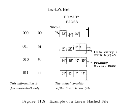
We have considerable flexibility in how to trigger a split, thanks to the use of overflow pages. We can split whenever a new overflow page is added, or we can impose additional conditions based all conditions such as space utilization. For our examples, a split is ‘triggered’ when inserting a new data entry causes the creation of an overftow page. Whenever a split is triggered the Next bucket is split, and hash function $h_{level + 1}$ redistributes entries between this bucket (say bucket number b) and its split image; the split image is therefore bucket number b + $N_{level}$. After splitting a bucket, the value of Next is incremented by 1. In the example file, insertion of data entry 43* triggers a split. The file after completing the insertion is shown in Figure 11.9.

At any time in the middle of a round Level, all buckets above bucket Next have been split, and the file contains buckets that are their split images, as illustrated in Figure 11.7. Buckets Next through $N_{level}$ have not yet been split. If we use $h_{level}$ on a data entry and obtain a number b in the range Next through $N_{level}$, the data entry belongs to bucket b. For example, $h_0(18)$ is 2 (binary 10); since this value is between the current values of Next (= 1) and $N_1$ (=4), this bucket has not been split. However, if we obtain a number b in the range 0 through Next, the data entry may be in this bucket or in its split image (which is bucket number $b+N_{level}$; we have to use $h_{level}+1$ to determine to which of these two buckets the data entry belongs. In other words, we have to look at one more bit of the data entry’s hash value. For example, $h_0(32)$ and $h_0(44)$ are both a (binary 00). Since Next is currently equal to 1, which indicates a bucket that has been split, we have to apply $h_1$. We have $h_1$ (32) = 0 (binary 000) and $h_1$ (44) = 4 (binary 100). Therefore, 32 belongs in bucket A and 44 belongs in its split image, bucket A2. Not all insertions trigger a split, of course. If we insert 37* into the file shown in Figure 11.9, the appropriate bucket has space for the new data entry. The file after the insertion is shown in Figure 11.10.

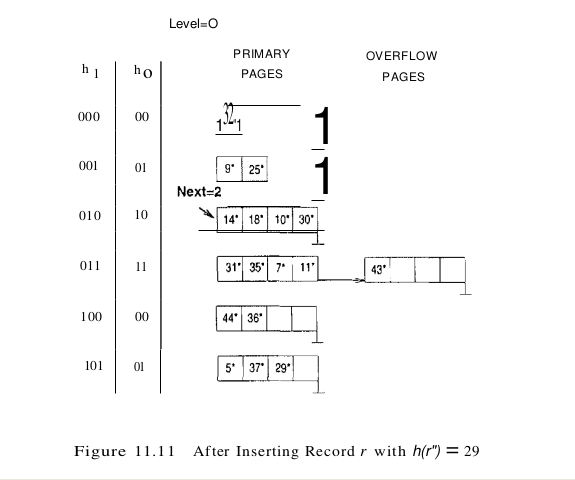
Sometimes the bucket pointed to by Next (the current candidate for splitting) is full, and a new data entry should be inserted in this bucket. In this case, a split is triggered, of course, but we do not need a new overflow bucket. This situation is illustrated by inserting 29* into the file shown in Figure 11.10. The result is shown in Figure 11.11.
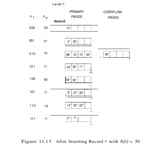
When Next is equal to $N_{level} - 1$ and a split is triggered, we split the last of the buckets present in the file at the beginning of round Level. The number of buckets after the split is twice the number at the beginning of the round, and we start a new round with Level incremented by 1 and Next reset to O. Incrementing Level amounts to doubling the effective range into which keys are hashed. Consider the example file in Figure 11.12, which was obtained from the file of Figure 11.11 by inserting 22*, 66*, and 34*. (The reader is encouraged to try to work out the details of these insertions.) Inserting 50* causes a split that leads to incrementing Level, as discussed previously; the file after this insertion is shown in Figure 11.13.

In summary, an equality selection costs just one disk I/O unless the bucket has overflow pages; in practice, the cost on average is about 1.2 disk accesses for reasonably uniform data distributions. (The cost can be considerably worse–linear in the number of data entries in the file–if the distribution is very skewed. The space utilization is also very poor with skewed data distributions.) Inserts require reading and writing a single page, unless a split is triggered. We do not discuss deletion in detail, but it is essentially the inverse of insertion. If the last bucket in the file is empty, it can be removed and Next can be decremented. (If Next is 0 and the last bucket becomes empty, Next is made to point to bucket (M /2) - 1, where M is the current number of buckets, Level is decremented, and the empty bucket is removed.) If we wish, we can combine the last bucket with its split image even when it is not empty, using some criterion to trigger this merging in essentially the same way. The criterion is typically based on the occupancy of the file, and merging can be done to improve space utilization.
Extendible VS Linear Hashing
To understand the relationship between Linear Hashing and Extendible Hashing, imagine that we also have a directory in Linear Hashing with elements 0 to N - 1. The first split is at bucket 0, and so we add directory element N. In principle, we may imagine that the entire directory has been doubled at this point; however, because element 1 is the same as element N + 1, element 2 is the same as element N + 2, and so on, we can avoid the actual copying for the rest of the directory. The second split occurs at bucket 1; now directory element N + 1 becomes significant and is added. At the end of the round, all the original N buckets are split, and the directory is doubled in size (because all elements point to distinct buckets).
We observe that the choice of hashing functions is actually very similar to what goes on in Extendible Hashing–in effect, moving from $h_i$ to $h_{i + 1}$ in Linear Hashing corresponds to doubling the directory in Extendible Hashing. Both operations double the effective range into which key values are hashed; but whereas the directory is doubled in a single step of Extendible Hashing, moving from $h_i$ to $h_{i + 1}$, along with a corresponding doubling in the number of buckets, occurs gradually over the course of a round in Linear Hashing. The new idea behind Linear Hashing is that a directory can be avoided by a clever choice of the bucket to split. On the other hand, by always splitting the appropriate bucket, Extendible Hashing may lead to a reduced number of splits and higher bucket occupancy. The directory analogy is useful for understanding the ideas behind Extendible and Linear Hashing. However, the directory structure can be avoided for Linear Hashing (but not for Extendible Hashing) by allocating primary bucket pages consecutively, which would allow us to locate the page for bucket i by a simple offset calculation. For uniform distributions, this implementation of Linear Hashing has a lower average cost for equality selections (because the directory level is eliminated). For skewed distributions, this implementation could result in any empty or nearly empty buckets, each of which is allocated at least one page, leading to poor performance relative to Extendible Hashing, which is likely to have higher bucket occupancy. A different implementation of Linear Hashing, in which a directory is actually maintained, offers the flexibility of not allocating one page per bucket; null directory elements can be used as in Extendible Hashing. However, this implementation introduces the overhead of a directory level and could prove costly for large, uniformly distributed files. (Also, although this implementation alleviates the potential problem of low bucket occupancy by not allocating pages for empty buckets, it is not a complete solution because we can still have many pages with very few entries.)